College aantekeningen

Lecture notes theme statistics Clinical Research in Practise (CRIP)

1 keer verkocht

Instelling
Universiteit Leiden (UL)

Complete lecture notes of the theme statistics in the course Clinical Research in Practice (CRIP) of the master Biomedical Sciences at the LUMC. Lecturers from Bart Mertens.

[Meer zien]

Voorbeeld 2 van de 5 pagina's

Bekijk voorbeeld

Geupload op 19 oktober 2022
Aantal pagina's 5
Geschreven in 2022/2023
Type College aantekeningen
Docent(en) Bart mertens
Bevat All lectures theme statistics

statistics
linear regression
survival
logistic regression
p value
odds ratio
hazard ratio
mixed models
models
deviance
hazard
survival probability
cox regression
kaplan meier
r

€3,19

In winkelwagen

Op verlanglijstje

100% tevredenheidsgarantie
Direct beschikbaar na je betaling
Lees online óf als PDF
Geen vaste maandelijkse kosten

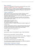
Basic statistics
oddsratio (table): calculate odds ratio, the odds ratio can be found in the ‘measure’ section
Unpaired t test in R studio: t.test (y ~ x, data=…, var.equal=TRUE)
When using var.equal=FALSE, the Welsh correction will be applied (for unequal variances)
It tests whether the difference between two groups is significant. First calculate the standard
error, then divide the difference by the standard error which gives the t value. When the t
value is >2 or <-2, the p value is <0,05.

Logistic regression
Logistic regression uses binary outcomes (has only 2 options: dichotomous outcome)
Binary outcomes are easily observed (e.g., death or not), it’s categorical data
Other types of categorical data are ordered (no response, low response, high response) and
unordered (red, blue, pink) outcomes
Death is a process that requires time (everyone dies eventually), so the time till death
(continuous data) is also often important; another option is to limit the observation time
(does the patient die within a month?)

In logistic regression, the outcome Y is 0 or 1
Classical regression is stated by: Y =α + β ∙ X+ ε
The  is the error variation of each measurement
The probability of outcome Y=1 is called p, and p depends on a predictor X (weight e.g.) 
p
ln ( )=α + β ∙ x
1−p
The data of a logistic regression can be put in a scatter plot which means that a line can be
drawn which says something about the relation between the variable and the outcome
(increasing line means positive effect (positive ), flat line means no effect).
p
The odds are defined as: odds= and odds=eα + β ∙ X
1− p
odds
Thus: p=
1+odds
eλ
When the logit () is known, p can be calculated by p= (= logistic transformation)
1+e λ

When you also have a binary predictor, a 2x2 table is easily made

Then  can be defined by the p when X=0 (p0) and when X=1 (p1): ln (
p1
1−p 1
)−ln
(p0
1−p 0 )
=β

since  defines the difference between the two predictors (the effect).
Hence, odds ratio=e β (for binary predictors)
α p0
For the odds in the reference/base group (), you say that e =
1− p0
For non-binary predictors, the regression effect  is the amount added to the log(odds) for
every unit increase in the predictor (e.g., 1 kg increase).

Fitting logistic regression models
Often, there’re multiple predictors. This means that the formula has multiple ’s.

, Model fitting = making a choice for the value of  and 
The ‘yardstick’ L defines how well the choice (suitability) for  and  is (the higher, the
better)
When you chose an  and , you can calculate the probability that would be calculated for
each observation that happened. If you do it right, the probabilities are true.
The choice for which the evidence is maximal is the maximum likelihood estimate α^ and ^β
In a likelihood contour plot, you plot  and . The darker the color, the better the estimate.

Model extension is needed when there needs to be corrected for another factor. After
adding another predictor, the two models should be compared to determine if you should
accept the new model for the same data or not (hypothesis testing). It is not univariate
testing: you test if there’s an effect of a second predictor while looking at another predictor.
The larger the difference between the L of the 2 models is, the better the extension is.
For this difference, we use the deviance = −2 ln (L). The difference is the first deviance
minus the second deviance (the deviance thus should be low).
The difference is distributed as X 2p (p is number of tested parameters). The p value is
obtained by comparing the deviance with the X 2p distribution.
This deviance testing is likelihood ratio testing (since it is evaluating the ratio of the
likelihoods)
The given standard error can be used to calculate the confidence interval of  by
± 1.96 ∙ s . e . (the whole thing e^… for the odds ratio)
^
❑−❑ 0
The null hypothesis is assessed by the z value: z= = Wald test (determine
s . e .( )
significance)

R: Logistic regression
glm (y ~ x, family=”binomial”, data =…)
Then save the model as a variable to use it for the command summary (…) which gives more
information (including  (estimate),  (intercept estimate), and the p value (Wald test))
Often, we are interested in the coefficients, so the command …$coefficients can be used
…$fitted.values gives the probability for each observation in the study
…$linear.predictors gives the value of +*x for each observation
Those two values can be plotted in a scatterplot which should be the same curve obtained by
plotting the predictor and the outcome. The probability is 0,5 at the linear predictor of 0.
Putting the x values on the x-axis instead of linear predictors gives the same curve.
Create a binary predictor (dichotomized variable) by … <- cut (…, breaks=c (…, …, …) (create 2
intervals)

anova (…) gives the difference of the null deviance and the residual deviance of a logistic
regression model (other test for significance). Multiple models can also be put in the
command.
The residual deviance is the deviance of the fitted (new) model. The null deviance is the
likelihood with no predictors at all.
Adding a factor in the logistic regression is done by the command glm (y ~ x1+x2,
family=”binomial”, data =…).
When the new factor has no effect, the deviance and the coefficient should not change
much.

Dit zijn jouw voordelen als je samenvattingen koopt bij Stuvia:

Bewezen kwaliteit door reviews

Studenten hebben al meer dan 850.000 samenvattingen beoordeeld. Zo weet jij zeker dat je de beste keuze maakt!

In een paar klikken geregeld

Geen gedoe — betaal gewoon eenmalig met iDeal, creditcard of je Stuvia-tegoed en je bent klaar. Geen abonnement nodig.

Direct to-the-point

Studenten maken samenvattingen voor studenten. Dat betekent: actuele inhoud waar jij écht wat aan hebt. Geen overbodige details!

Veelgestelde vragen

Wat krijg ik als ik dit document koop?

Je krijgt een PDF, die direct beschikbaar is na je aankoop. Het gekochte document is altijd, overal en oneindig toegankelijk via je profiel.

Tevredenheidsgarantie: hoe werkt dat?

Onze tevredenheidsgarantie zorgt ervoor dat je altijd een studiedocument vindt dat goed bij je past. Je vult een formulier in en onze klantenservice regelt de rest.

Van wie koop ik deze samenvatting?

Stuvia is een marktplaats, je koop dit document dus niet van ons, maar van verkoper verabw. Stuvia faciliteert de betaling aan de verkoper.

Zit ik meteen vast aan een abonnement?

Nee, je koopt alleen deze samenvatting voor €3,19. Je zit daarna nergens aan vast.

Is Stuvia te vertrouwen?

4,6 sterren op Google & Trustpilot (+1000 reviews)

Afgelopen 30 dagen zijn er 68175 samenvattingen verkocht

Opgericht in 2010, al 15 jaar dé plek om samenvattingen te kopen

Begin nu gratis