Overig

APM3711 Numerical Methods II

7 keer verkocht

Vak
MAT3701 Linear Algebra

Instelling
University Of South Africa (Unisa)

APM3711 Numerical Methods III is a third year UNISA module that focuses on problem solving and critical thinking. Its pre-requisite module is APM2613. Its purpose is to equip students with numerical techniques for the approximate solution of initial and boundary value problems of differential equat...

[Meer zien]

Voorbeeld 4 van de 347 pagina's

Bekijk voorbeeld

Geupload op 7 november 2022
Aantal pagina's 347
Geschreven in 2021/2022
Type Overig
Persoon Onbekend

exam preparation
solutions
revision material
apm3711 numerical methods ii

Instelling
University of South Africa (Unisa)
Vak
MAT3701 Linear Algebra

€3,75

Ook beschikbaar in voordeelbundel v.a. €9,64

In winkelwagen

Op verlanglijstje

100% tevredenheidsgarantie
Direct beschikbaar na je betaling
Lees online óf als PDF
Geen vaste maandelijkse kosten

Ook beschikbaar in voordeelbundel (1)

APM3711 AND MAT3701 PREVIOUS ASSIGNMENTS AND EXAMS

€ 12,32 € 9,64 3 items

1. Overig - Apm3711 numerical methods ii
2. Overig - Mat3701 - linear algebra iii
3. Tentamen (uitwerkingen) - Mat3701 linear algebra exam revision material
Meer zien

ADDENDUM A: Assignments
A.1 Assignment 01

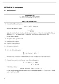
ASSIGNMENT 01
Due date: Wednesday, 20 April 2022

ONLY FOR YEAR MODULE

1. Consider the differential equation

y 0 (x) = −3x 2 y 2 , y(0) = 2,

which has the analytical solution
2
y= .
2x 3 + 1
Apply the modified Euler method to solve the equation up to x = 1 first with steplength h = 0.2 and
then with h = 0.1. At each step make 2 corrections. Also calculate the error at each step.
In your solution include:

(i) description of the algorithms used

(ii) program listing (printout)

(iii) computer results (printout)

(iv) discussion of the results

2. Solve the differential equation
dy
= 3x + 2y + xy, y(0) = −1
dx

by means of the Taylor-series expansion to get the value of y at x = 0.1. Use terms up to x 6 .

3. Consider the system of coupled second-order differential equations

u 00 − (t + 1)uv + v 0 = cos t
v 00 = u 0 + uv

with initial conditions
u(0) = 2, u 0 (0) = 1, v (0) = 3, v 0 (0) = −1.
Use the second-order Runge-Kutta method with h = 0.2 and a = 2/3, b = 1/3, α = β = 3/2, to find
u, u 0 , v and v 0 at t = 0.2.

14

, APM3711/101/0/2022

A.2 Assignment 02

ASSIGNMENT 02
Due date: Monday, 30 May 2022

ONLY FOR YEAR MODULE

1. For the equation
y 0 = y sin (πx) , y(0) = 1,
get starting values by the Runge-Kutta Fehlberg method for x = 0.2, x = 0.4, x = 0.6, and then
advance the solution to x = 1.0 by

(a) Milne’s method,
(b) the Adams-Moulton method.

2. Solve the boundary–value problem

y 00 + x 2 y 0 − 4xy = 2x 3 + 6x 2 − 2, y(0) = 0, y(1) = 2

by using the shooting method. Use the modified Euler method (with only one correction at
each step), and take h = 0.2. Start with an initial slope of y 0 (0) = 1.9 as a first attempt and
y 0 (0) = 2.1 as a second attempt. Then interpolate.
Compare the result with the analytical solution y = x 4 − x 2 + 2x.

3.
(a) The function ex is to be approximated by a fifth-order polynomial over the interval [−1, 1]. Why
is a Chebyshev series a better choice than a Taylor (or Maclaurin) expansion?
(b) Given the power series
f (x) = 1 − x − 2x 3 − 4x 4
and the Chebyshev polynomials

T0 (x) = 1
T1 (x) = x
T2 (x) = 2x 2 − 1
T3 (x) = 4x 3 − 3x
T4 (x) = 8x 4 − 8x 2 + 1,

economize the power series f (x) twice.
(c) Find the Padé approximation R2 (x), with numerator of degree 2 and denominator of degree 1, to
the function f (x) = x 2 + x 3 .

15

, ASSIGNMENT 03
Due date: Monday, 20 June 2022

ONLY FOR YEAR MODULE

1. Solve the boundary–value problem

y 00 + x 2 y 0 − 4xy = 2x 3 + 6x 2 − 2, y (0) = 0, y(1) = 2

by using the shooting method. Use the modified Euler method (with only one correction at each step),
and take h = 0.2. Start with an initial slope of y 0 (0) = 1.9 as a first attempt and y 0 (0) = 2.1 as a
second attempt. Then interpolate.
Compare the result with the analytical solution y = x 4 − x 2 + 2x.

2. (a) Define what is meant by the eigenvalues and eigenvectors of a matrix A.
If the matrix A is  
2 0 1
A =  −22 −3 10  ,
−12 0 9

(b) find the characteristic polynomial,
(c) find the eigenvalues and eigenvectors.
(d) Start with the approximate eigenvector (1,1,1) and use the power method to estimate the dominant
eigenvalue by iterating 4 times.
(e) Use the power method to find the smallest absolute eigenvalue of A.
(f) Write a program which applies the power method to a given matrix in (d) and (e) above.

3. Consider the following boundary–value problem:

y 00 = 2x 2 y 0 + xy + 2, 1 ≤ x ≤ 4.

Taking h = 1, set up the set of equations required to solve the problem by the finite difference method
in each of the following cases of boundary conditions:

(a) y(1) = −1, y(4) = 4;
(b) y 0 (1) = 2, y 0 (4) = 0;
(c) y 0 (1) = y(1), y 0 (4) = −2y(4).

(Do not solve the equations!).

16

, APM3711/101/0/2022

ASSIGNMENT 04
Due date: Friday, 29 July 2022

ONLY FOR YEAR MODULE
1. Consider the partial differential equation
yu − 2∇2 u = 12, 0 < x < 4, 0 < y < 3
with boundary conditions
x = 0 and x = 4 : u = 60
∂u
y = 0 and y = 3 : = 5.
∂y
(a) Taking h = 1, sketch the region and the grid points. Use symmetry to minimize the number of
unknowns ui that have to be calculated and indicate the ui in the sketch.
(b) Use the 5-point difference formula for the Laplace operator to derive a system of equations for
the ui .

2. We have a plate of 12 × 15 cm and the temperatures on the edges are held as shown in the sketch
below. Take ∆x = ∆y = 3 cm and use the S.O.R. method (successive overrelaxation method) to find
the temperatures at all the grid points. First calculate the optimal value of ω and then use this value in
the algorithm. Start with all grid values equal to the arithmetic average of the given boundary values.

3. Solve the problem in question 2 by using the A.D.I method (alternating-direction-implicit method)
without overrelaxation.

17

Dit zijn jouw voordelen als je samenvattingen koopt bij Stuvia:

Bewezen kwaliteit door reviews

Studenten hebben al meer dan 850.000 samenvattingen beoordeeld. Zo weet jij zeker dat je de beste keuze maakt!

In een paar klikken geregeld

Geen gedoe — betaal gewoon eenmalig met iDeal, creditcard of je Stuvia-tegoed en je bent klaar. Geen abonnement nodig.

Direct to-the-point

Studenten maken samenvattingen voor studenten. Dat betekent: actuele inhoud waar jij écht wat aan hebt. Geen overbodige details!

Veelgestelde vragen

Wat krijg ik als ik dit document koop?

Je krijgt een PDF, die direct beschikbaar is na je aankoop. Het gekochte document is altijd, overal en oneindig toegankelijk via je profiel.

Tevredenheidsgarantie: hoe werkt dat?

Onze tevredenheidsgarantie zorgt ervoor dat je altijd een studiedocument vindt dat goed bij je past. Je vult een formulier in en onze klantenservice regelt de rest.

Van wie koop ik deze samenvatting?

Stuvia is een marktplaats, je koop dit document dus niet van ons, maar van verkoper znyele. Stuvia faciliteert de betaling aan de verkoper.

Zit ik meteen vast aan een abonnement?

Nee, je koopt alleen deze samenvatting voor €3,75. Je zit daarna nergens aan vast.

Is Stuvia te vertrouwen?

4,6 sterren op Google & Trustpilot (+1000 reviews)

Afgelopen 30 dagen zijn er 67418 samenvattingen verkocht

Opgericht in 2010, al 15 jaar dé plek om samenvattingen te kopen

Begin nu gratis