100% tevredenheidsgarantie Direct beschikbaar na betaling Zowel online als in PDF Je zit nergens aan vast
logo-home
Data Analysis and Visualisation Summary €8,44   In winkelwagen

Samenvatting

Data Analysis and Visualisation Summary

1 beoordeling
 368 keer bekeken  17 keer verkocht

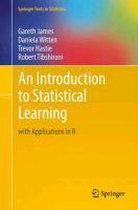
This is a summary of the Data Analysis and Visualisation course taught at Utrecht University as part of the Applied Data Science (ADS) profile. Its contents are an extensive yet comprehensive summary of all chapters of the book Introduction to Statistical Learning (James et al.) and relevant papers...

[Meer zien]

Voorbeeld 10 van de 41  pagina's

  • Nee
  • 1, 2, 3, 4, 5, 6, 7, 8, 10
  • 6 maart 2018
  • 41
  • 2017/2018
  • Samenvatting
book image

Titel boek:

Auteur(s):

  • Uitgave:
  • ISBN:
  • Druk:
Alle documenten voor dit vak (1)

1  beoordeling

review-writer-avatar

Door: Tije • 5 jaar geleden

avatar-seller
KNiemeijer
DATA ANALYSIS &
VISUALISATION

Summary of Data Analysis & Visualisation 2017 course (201600038) from
Utrecht University


Koen Niemeijer

,Contents
Week 1: Data Analysis................................................................................................. 3
Week 2: Exploratory Data Analysis ............................................................................ 4
Univariate non-graphical ........................................................................................ 4
Univariate graphical ................................................................................................ 4
Multivariate non-graphical ..................................................................................... 4
Multivariate graphical ............................................................................................. 4
Week 3: Linear Regression .......................................................................................... 5
3. Linear Regression ................................................................................................. 5
3.1.2 Assessing the Accuracy of the Coefficient Estimates ............................ 7
3.2 Multiple Linear Regression ............................................................................. 8
3.2.2 Some important questions ......................................................................... 8
3.3.1 Qualitative Predictors ................................................................................. 9
3.3.2 Extension of the Linear Model ................................................................... 9
3.3.3 Potential problems .................................................................................... 10
3.4 Possible questions and answers ................................................................. 11
3.5 Comparison of Linear Regression with K-Nearest Neighbours ............... 11
6. Linear Model Selection and Regularisation ................................................... 12
Week 4 & 5: Resampling and Non-Linear Regression........................................... 13
5. Resampling methods......................................................................................... 13
5.1 Cross-Validation ........................................................................................... 13
5.2 The Bootstrap ................................................................................................ 14
7. Moving Beyond Linearity .................................................................................. 14
7.1 Polynomial Regression ................................................................................. 14
7.2 Step Functions .............................................................................................. 14
7.3 Basis Functions .............................................................................................. 15
7.4 Regression splines ......................................................................................... 15
7.5 Smoothing Splines ........................................................................................ 16
7.6 Local Regression........................................................................................... 16
7.7 Generalised Additive Models ..................................................................... 17
8. Tree-Based Methods.......................................................................................... 18
8.1.1 Regression Trees ........................................................................................ 18
8.1.4 Advantages and Disadvantages of Trees ............................................. 19
8.2.1 Bagging ...................................................................................................... 20
8.2.2 Random Forests ......................................................................................... 20


Koen Niemeijer Data Analysis & Visualisation 1/40

, 8.2.3 Boosting ...................................................................................................... 20
Week 6: Classification ............................................................................................... 21
2.2.3 The classification Setting .............................................................................. 21
4. Classification ....................................................................................................... 22
4.2 Why Not Linear Regression? ....................................................................... 22
4.3 Logistic Regression ....................................................................................... 22
4.4 Linear Discriminant Analysis ........................................................................ 23
4.5 A Comparison of Classification Methods ................................................. 25
5.1.5 Cross-Validation on Classification Problems ............................................. 26
Week 7: Trees ............................................................................................................. 26
8. Tree-Based Methods.......................................................................................... 26
8.1.2 Classification Trees .................................................................................... 26
8.1.3 Trees Versus Linear Models....................................................................... 27
Week 8: Principle Component Analysis .................................................................. 27
10. Unsupervised Learning .................................................................................... 27
10.2 Principle Component Analysis.................................................................. 27
Greenacre 8: Correspondence Analysis Biplots ................................................ 29
Week 9: Cluster Analysis ........................................................................................... 31
10.3 Clustering Methods........................................................................................ 31
10.3.1 K-Means Clustering ................................................................................. 31
10.3.2 Hierarchical Clustering ........................................................................... 32
10.3.3 Practical Issues in Clustering .................................................................. 34
Kumar 8: Cluster Analysis: Basic Concepts and Algorithms ............................. 34
8.1 Overview ....................................................................................................... 35
8.2: K-Means ........................................................................................................ 36
Formulae ..................................................................................................................... 38


Koen Niemeijer Data Analysis & Visualisation 2/40

,Week 1: Data Analysis
Data analysis goals:
• Description
• Prediction
• Explanation
• Prescription

Data analysis modes:
• Exploratory
• Confirmatory


Exploratory data analysis: Describing interesting patterns: use graphs,
summaries, to understand subgroups, detect anomalies (“outliers”),
understand the data.
• Supervised learning:
o Regression: predict continuous labels from other values.
o Classification: predict discrete labels from other values.
• Unsupervised learning: Classify or predict unknown values.
o Clustering, Low rank matrix decomposition, PCA, multiple
correspondence analysis.


There are many names for data analysis (data modelling, machine learning,
statistical learning), but in practice people often do not know the difference.


Koen Niemeijer Data Analysis & Visualisation 3/40

,As such, we can treat them as the same process even though they are not
exact synonyms.

We need data analysis and data visualisation because data analysis and the
accompanying visualizations have yielded insights and solved problems that
could not be solved without them.


Week 2: Exploratory Data Analysis
Four types of EDA:
Univariate non-graphical
• A simple tabulation of the frequency of each category
• Histogram

The central tendency or “location” of a distribution has to do with typical or
middle values.
• Mean
o Parameter: Fixed mean for finite population
o Sampling distribution: Probability distribution of sample mean
• Median
o Robustness: Moving some data tends not to change the value of
the statistic.
• Mode

The variance is the mean of the squares of the individual deviations. The
standard deviation is the square root of the variance. The interquartile range
(IQR) is a robust measure of spread where IQR = Q3 – Q1 i.e. the middle 50%.
Skewness is a measure of asymmetry. Kurtosis is a more subtle measure of
peakedness compared to a Gaussian distribution.
Univariate graphical
• Histogram
• Stem-and-leaf plot
• Boxplot
• Quantile-normal plots allow detection of non-normality and diagnosis of
skewness and kurtosis.
Multivariate non-graphical
• Cross-tabulation
• Univariate statistics by category
• Covariance and correlation
• Covariance and correlation matrices
Multivariate graphical
• Side-by-side boxplots
• Scatterplots

Degrees of freedom are numbers that characterize specific distributions in a
family


Koen Niemeijer Data Analysis & Visualisation 4/40

,of distributions.

Things to look for when performing EDA:
• Typical values
o Which values are the most common? Why?
o Which values are rare? Why? Does that match your expectations?
o Can you see any unusual patterns? What might explain them?
• Unusual values


Week 3: Linear Regression
3. Linear Regression
Regression can be represented as 𝑌 = 𝑓(𝑋) + ϵ where there is some relationship
between Y and 𝑋 = (𝑋1 , 𝑋2 , … , 𝑋𝑝 ) and 𝜖 is a random error term. In this
formulation, f represents the systematic information that X provides about Y.
The error terms have approximately mean zero.

When predicting Y, the error is reducible by applying statistical learning
techniques. The error is irreducible since Y is also a function of 𝜖, which cannot
be predicted by X.

Regression can be used for:
• Predicting: Looking at how Y relates to X, without being concerned
which part of X influence Y. This is treating X as a black box.
• Inference: Being interested in how parts of X influence Y.

Most statistical learning methods for this task can be characterised as either
parametric or non-parametric.
• Parametric: Make a regression in 2 steps. (1) make assumptions about
the linear form and choose a regression model, and (2) create
parameters for each 𝑋𝑛 so that it the line fits the model.
o Overfitting: when the line follows the noise (errors) too closely
• Non-parametric: doesn’t make any assumptions about f and is therefore
better than a parametric approach. However, it does need a very large
number of observations in order to accurately estimate f. Hence, there
is a danger of overfitting f by not being smooth enough.

Restrictive approaches are preferable over flexible approach when the goal is
interpretability:


Koen Niemeijer Data Analysis & Visualisation 5/40

,Supervised learning: when the outcome Y is known and you’re able to make
predictions.
Unsupervised learning: outcome Y is unknown and you’re trying to find patterns
in the data.
Semi-supervised learning: when some measurements are available, and some
are not.

1
Mean squared error ∑𝑛𝑖=1(𝑦𝑖 − 𝑓̂(𝑥𝑖 ))2 is computed using the training data used
𝑛
to fit the model. But in general, we do not really care how well the method
works on the training data. Rather, we are interested in the accuracy of the
pre- MSE predictions that we obtain when we apply our method to previously
unseen test data.

As the flexibility of the model increases, the training MSE will decrease but a
large test MSE may not. When a given method yields a small training MSE but a
large test MSE, we are said to be overfitting the data.

it is possible to show that the expected test MSE, for a given value x0, can
always be decomposed into the sum of three fundamental quantities: the
variance of 𝑓̌(𝑥0 ), the squared bias of 𝑓̌(𝑥0 ), and the variance of the error terms
𝜖.
 Test MSE can never lie below irreducible error
 In order to get low test MSE, you need get a statistical learning
method with low bias and low variance

Synergy / Interaction effect: when two variables interact to create an effect.
Together they are called coefficients or parameters. When Y is modelled onto
X:
𝑌 ≈ 𝛽0 + β1 𝑋


Koen Niemeijer Data Analysis & Visualisation 6/40

,The coefficient β0 is the intercept and β1 is the slope of the linear model. To
estimate the parameters, we can use the sum of squares (RSS):
2 2 2
𝑅𝑆𝑆 = (𝑦1 − β̂0 − β̂1 x1 ) + (𝑦2 − β̂0 − β̂1 x2 ) + (𝑦1 − β̂0 − β̂1 xn )


3.1.2 Assessing the Accuracy of the Coefficient Estimates
The population regression line is the best linear approximation to the true
relationship between X and Y. The least squares regression coefficient estimates
characterise the least squares line.

Unbiased versus biased estimate: an estimate with an average μ̂ will something
over- sometimes underestimate μ , but on overage it will exactly equal μ
provided enough attempts. However, if an estimate is biased (comes from the
same data set) it might be the case that the data set is different from the
population.
σ2
𝑉𝐴𝑅(μ̂) = 𝑆𝐸(μ̂2 ) =
𝑛
To estimate how for β̂0 is off from μ̂:
2 1 𝑥̅ 2 2 σ2
𝑆𝐸(β̂0 ) = σ2 [ + ∑𝑛 2 ], SE(β̂0 ) = [∑𝑛 2 ] where σ2 = 𝑉𝑎𝑟(ϵ).
𝑛 𝑖=1(𝑥𝑖 −𝑥̅ ) 𝑖=1(𝑥𝑖 −𝑥̅ )


The estimate of σ is known as the residual standard error, and is given by the
formula
𝑅𝑆𝐸 = √𝑅𝑆𝑆/(𝑛 − 2)
Standard errors can be used to compute confidence intervals. For linear
regression, the confidence interval of 95% corresponds to 2 * SE

In singular linear regression models, the hypotheses are:
𝐻0 : β1 = 0
𝐻1 : β1 ≠ 0

To test if the alternative hypothesis differs from the null hypothesis, a t-test can
̂ 1 −0
β
be performed: 𝑡 = ̂1) which measures the number of standard deviations
𝑆𝐸(β
that β1 is away from 0.

3.1.3 Assessing the Accuracy of the Model
The residual standard error is the average amount that the response will
1 1
deviate from the true regression line: 𝑅𝑆𝐸 = √ 𝑅𝑆𝑆 =√ ∑𝑛 (𝑦 − 𝑦2 )2 . The
𝑛−2 𝑛−2 𝑖=1 1
RSE is considered a measure of the lack of fit of the model to the data.

Absolute values aren’t always a good measure for lack of fit. 𝑅 2 measures in
proportions:
𝑇𝑆𝑆−𝑅𝑆𝑆 𝑅𝑆𝑆
𝑅2 = =1− where 𝑇𝑆𝑆 = ∑(𝑦𝑖 − 𝑦̅)2 is the total sum of squares.
𝑇𝑆𝑆 𝑇𝑆𝑆


Koen Niemeijer Data Analysis & Visualisation 7/40

,An 𝑅 2 statistic that is close to 1 indicates that a large proportion of the
variability in the response has been explained by the regression. A number near
0 indicates that the regression did not explain much of the variability in the
response; this might occur because the linear model is wrong, or the inherent
error σ2 is high, or both.

∑𝑛
𝑖=1(𝑥𝑖 −𝑥̅ )(𝑦𝑖 −𝑦
̅)
In univariate linear regression, 𝑅 2 = 𝑟 2 , where 𝐶𝑜𝑟 =
√∑𝑛 2 ̅2)
𝑖=1(𝑥1 −𝑥̅ ) √∑𝑖=1 𝑛(𝑦𝑖 −𝑦

3.2 Multiple Linear Regression
Addresses the problem of creates regressions with multiple predictors. Multiple
regressions with single predictors are not satisfactory as they do not show the
interaction between independent variables. In case of multiple linear
regression, the formula is
𝑌 = β0 + β1 𝑋1 + β2 𝑋2 + ⋯ + β𝑝 𝑋𝑝 + ϵ
Parameters are estimated using the least squares approach. β0 , β1 , … , β𝑝 are
chosen to minimise the sum of squared residuals:
𝑛

𝑅𝑆𝑆 = ∑(𝑦𝑖 − 𝑦̂𝑖 )2
𝑖=1
Multiple linear regression is able to filter out the effects of predictors on the
outcome that actually have no effect, but take ‘credit’ from other predictors.

3.2.2 Some important questions
1. Is at least one of the predictors X1, X2,...,Xp useful in predicting
the response?
In multiple linear regression, the hypotheses are:
𝐻0 : β1 = β2 = ⋯ = β𝑝 = 0
𝐻1 : at least some β𝑗 is non − zero

This hypothesis test is performed by computing the F-statistic,
(𝑇𝑆𝑆 − 𝑅𝑆𝑆)/𝑝
𝐹=
𝑅𝑆𝑆/(𝑛 − 𝑝 − 1)
The significance of F depends on p and n. Looking at every predictor
individually to look for significance doesn’t work, especially when p is large. The
overall F-statistic takes this into account by being able to filter out a particular
factor:
(𝑅𝑆𝑆0 − 𝑅𝑆𝑆)/𝑞
F=
𝑅𝑆𝑆/(𝑛 − 𝑝 − 1)
Where q is a subset of coefficients.

2. Do all the predictors help to explain Y , or is only a subset of the
predictors useful?
If questions 1 answers with yes (some predictor is related to the response), then
find out which one. Variable selection creates subsets of predictors to see
which one is related. However, this is infeasible. Other options:
• Forward selection: Start with null model, fit p predictors to regression,
add p to model that is most significant.


Koen Niemeijer Data Analysis & Visualisation 8/40

, • Backward selection: Start with all predictors, remove p that is least
significant.
• Mixed selection: Start with forward selection, go backwards when p gets
too large.

3. How well does the model fit the data?
In univariate linear regressions, 𝑅 2 = 𝑟 2 . However, in multiple linear regressions
2
𝑅 2 = 𝐶𝑜𝑟(𝑌, 𝑌̂) . An 𝑅 2 value close to 1 indicates that the model explains a large
portion of the variance in the response variable. 𝑅 2 always increases when
another predictor is added. As such, only a small increase may imply that it is
only weakly related and may be dropped. This is also true for RSE.

4. Given a set of predictor values, what response value should we predict, and
how accurate is our prediction?
Three uncertainties when predicting:
1. Coefficient is related to reducible error, though it is possible to compute
a confidence interval.
2. A linear model is (almost) always an estimation of the truth, so there is
an additional source of potentially reducible error which we will call
model bias. In other words, using a linear model is an assumption itself.
3. There is irreducible error ϵ which we cannot predict. It’s possible to use
prediction intervals, which are wider than confidence intervals because
they are both errors.

3.3.1 Qualitative Predictors
Qualitative predictors are called factors. They can be assigned a dummy
variable that takes on numerical values to represent them in coefficients. For
example:
1 if ith person is female
𝑥𝑖 = {
0 if ith person is male
β0 + β1 + ϵ𝑖
𝑦𝑖 = β0 + β1 𝑥1 + ϵ𝑖 = {
β0 + ϵ𝑖

When there are multiple levels in factors, additional levels can be added
through extra dummy variables. There will always be one fewer dummy
variable than the number of levels. This level with no dummy variable is known
as the baseline.

3.3.2 Extension of the Linear Model
Linear regression is based on two assumptions:
• Additive: the effect of changes in a predictor 𝑋𝑗 on the response Y is
independent of the values of the other predictors.
• Linear: the change in the response Y due to a one-unit change in 𝑋𝑗 is
constant, regardless of the value of 𝑋𝑗 .
One possibility to diminish the additive assumption, is to add an extra
parameter to the model which describes the interaction effects between
variables, i.e. 𝑌 = 𝛽0 + 𝛽1 𝑋1 + 𝛽2 𝑋2 + 𝛽3 𝑋1 𝑋2 + ϵ.


Koen Niemeijer Data Analysis & Visualisation 9/40

Voordelen van het kopen van samenvattingen bij Stuvia op een rij:

Verzekerd van kwaliteit door reviews

Verzekerd van kwaliteit door reviews

Stuvia-klanten hebben meer dan 700.000 samenvattingen beoordeeld. Zo weet je zeker dat je de beste documenten koopt!

Snel en makkelijk kopen

Snel en makkelijk kopen

Je betaalt supersnel en eenmalig met iDeal, creditcard of Stuvia-tegoed voor de samenvatting. Zonder lidmaatschap.

Focus op de essentie

Focus op de essentie

Samenvattingen worden geschreven voor en door anderen. Daarom zijn de samenvattingen altijd betrouwbaar en actueel. Zo kom je snel tot de kern!

Veelgestelde vragen

Wat krijg ik als ik dit document koop?

Je krijgt een PDF, die direct beschikbaar is na je aankoop. Het gekochte document is altijd, overal en oneindig toegankelijk via je profiel.

Tevredenheidsgarantie: hoe werkt dat?

Onze tevredenheidsgarantie zorgt ervoor dat je altijd een studiedocument vindt dat goed bij je past. Je vult een formulier in en onze klantenservice regelt de rest.

Van wie koop ik deze samenvatting?

Stuvia is een marktplaats, je koop dit document dus niet van ons, maar van verkoper KNiemeijer. Stuvia faciliteert de betaling aan de verkoper.

Zit ik meteen vast aan een abonnement?

Nee, je koopt alleen deze samenvatting voor €8,44. Je zit daarna nergens aan vast.

Is Stuvia te vertrouwen?

4,6 sterren op Google & Trustpilot (+1000 reviews)

Afgelopen 30 dagen zijn er 72042 samenvattingen verkocht

Opgericht in 2010, al 14 jaar dé plek om samenvattingen te kopen

Start met verkopen
€8,44  17x  verkocht
  • (1)
  Kopen