Lecture 1 + 2 (maths: 04-02 + 07-2) -> Ch. 1 + 2 + 7
Note: Maths (lecture 1+2) not required for exam
Chapter 1
Establish relationship between dependent (y) and explanatory (x) variables.
• Simple regression analysis – Using one explanatory variable;
• Multiple regression analysis – Using several explanatory variables.
The theoretical relationship between two or more variables in economics is derived from
economic theory. Economics often studies cause-effect relationships. It is often not always
clear however how strong this link is and whether this connection is i.e.
linear/quadratic/logarithmic etc.
The different functional forms are explained in the maths lectures.
• Relationship between dependent and explanatory variable can be:
o Linear;
o Log-linear;
o Quadratic.
% 𝑐ℎ𝑎𝑛𝑔𝑒 𝑦
• We calculate the first derivative (dy/dx) and elasticity (% 𝑐ℎ𝑎𝑛𝑔𝑒 𝑥 ) of the mathematical
functions.
Econometrics fills a gap between being an economics student and being a practicing
economist. We express out ideas about relationships between economic variables using
mathematical functions.
𝐶 = 𝑓(𝑌(𝑑)) – Consumptions as a function of disposable income.
𝑞 = 𝑓(𝑝, 𝑝(𝑠), 𝑝(𝑐), 𝑌(𝑑) – Demand for a specific type of car (i.e. Honda Civic) as a function of
its price, price of other cars (substitutes), complements and disposable income.
There is almost always variation differing the number of sold Honda Civics caused by its
dependent variables, hence a random stochastic component (e, error term) is added to the
regression equation to introduce all variation that can’t be explained by IV’s.
Regression (theoretical) – Purely abstract in nature, a way to model relations
econometrically:
• Multiple regression example: Y = β0 + β1p + β2ps + β3pc + β4Yd + e
• Single regression example 1: Y = β0 + β1X
o Slope, first derivative; (helling), is constant
• Single regression example 2: Y = β0 + β1X2
o Slope is not constant
• Error terms are in econometric models for several reasons:
o Many minor influences on Y are omitted from the equation;
o It is virtually impossible to avoid some sort of measurement error;
o The underlying theoretical model might have a different functional
form/shape than the one chosen for the regression (i.e. nonlinear);
o Human behaviour is (partially) unpredictable.
• Complete notation:
o Single linear regression model: Yi = β0 + β1Xi + εi
, o Multivariate (multiple) linear regression model: Yi = β0 + β1Xi + β2X2i + β3X3i
+ εi
o The i, is the amount of people in the sample (N). Every person has a different
beta (reaction on said X).
Estimated regression equation – Empirical best guesses of the true regression coefficients
βo + β1. They are obtained from data from a sample of Y-s and X-s. It has actual numbers for
the coefficients:
• Y̅i = 103.40 + 6.38X
o The hat on the Y is also on the coefficient terms (if not specified in numbers),
and shows that it is an estimation.
We can’t perform controlled experiments (a scientific test directly manipulated by a
scientist in order to test a single IV), so we rely on different forms of non-experimental
research (research that lacks the manipulation of an IV, or random assignment of
participants to conditions that have to be measured):
• Time series form → Data collected from discrete intervals during time.
• Cross section form → Data collected on a moment in time for a group of households
or firms.
• Panel data → A combination of both.
Chapter 2
Economic model example:
• S = βo + β1P + β2A
o S = Total sales in a week.
o P = Average price for the hamburgers chain.
▪ For this, you predict the following hypotheses:
• 𝐻0 : 𝛽 = 0
• 𝐻𝑎 : 𝛽 ≠ 0
▪ Higher price
o A = Advertising expenditure.
▪ For this, you predict the following hypotheses:
• 𝐻0 : 𝛽 ≤ 0
• 𝐻𝑎 : 𝛽 > 0
▪ More advertising leads to more sales.
• The thing you predict is what you put in your alternative hypothesis. With this, you are
going to test if this relation/prediction is also actually true.
o If it is significantly bigger than 0, you have enough reason to reject the null
hypothesis of no/negative relation.
Total Sum of Squares / Ordinary Least Squares (TSS/OLS) – The total sum of squares to
explain variation, divided in two parts: Variation that can be explained (ESS) and variation
that can’t be explained (RSS). It describes the overall fit of the estimated model, by
measuring the residual (= the difference between the observed value and the predicted
value for each error variable term).
, •
o
• By studying the model’s residuals we can determine the quality of the model and how
it can be improved if needed.
o To what extent it satisfies the OLS regression assumptions.
R2 (coefficient of determination) – Describes the overall fit of the estimated model. R2 = 87%
indicates that 87% of variation in total revenue is explained by the variation in price and the
variation in level of advertising expenditure (based on economic model).
2
𝐸𝑆𝑆 𝑅𝑆𝑆 𝛴𝑒 2 (𝑖) ∑(𝑌̅(𝑡)−𝑚𝑒𝑎𝑛(𝑌))
• 𝑇𝑆𝑆
; 1 − 𝑇𝑆𝑆
; 1 − ;
𝛴(𝑌𝑖−Ȳ)2 ∑(𝑌(𝑡)−𝑚𝑒𝑎𝑛(𝑌))2
o The third equation, and then the bottom 2nd Y is Ȳ.
• Problem: By adding more variables (making it a multivariate model), R2 will rise, even
if the variables added have no economic justification.
• Is always between 0 and 1.
Example:
, • The first model error term is nearly always lower (or in exceptional case equal) than
model 2’s error, implying that the R-squared is (almost) always higher in model 2 than
in model 1.
• In one scenario 𝑅 2 is equal → If alpha-3 equals exactly zero, then Q-3 is zero also, so
it is removed and both models are equal valued.
′
o Adding more variables increases 𝑅 2 𝑠 value → Meaning of this value is
limited.
o Hence 𝑅 2 is not used anymore when dealing with over 1 variable. For a
multivariate regression (over 1 IV) you use the adjusted 𝑅 2.
Adjusted R2(adj.) – Measures the % variation of Y around its mean explained by the
regression equation, adjusted for degrees of freedom.
𝐾
• Best formula: R2adj. = 𝑅 2 − [(𝑁−𝐾−1)] ∗ (1 − 𝑅 2 )
o N – Total number of observations.
o K – Number of explanatory variables (= IV) (excluding constant term).
o K+1 – Number of explanatory variables (including constant term).
• Alternative formulas:
𝑅𝑆𝑆
2 (𝑁−𝐾−1)
o 𝑅𝑎𝑑𝑗 =1− 𝑇𝑆𝑆
𝑁−1
o
• Two ways of denoting:
2
o 𝑅𝑎𝑑𝑗 or 𝑅̅ 2
• With the following data (we need N, K and 𝑅 2 to get 𝑅𝑎𝑑𝑗2
), we find both adjusted
values.
o Because model 2’s adjusted 𝑅 2 is higher, it is a better fit and better to use
than model 1.
o Apart from the (𝑎𝑑𝑗𝑢𝑠𝑡𝑒𝑑) 𝑅2 , you should also always look at the sign of the
coefficients (+/-) and see if it matches your prediction, and if the coefficient is
significant (t-value should be bigger than the critical t-value).
Note: Maths (lecture 1+2) not required for exam
Chapter 1
Establish relationship between dependent (y) and explanatory (x) variables.
• Simple regression analysis – Using one explanatory variable;
• Multiple regression analysis – Using several explanatory variables.
The theoretical relationship between two or more variables in economics is derived from
economic theory. Economics often studies cause-effect relationships. It is often not always
clear however how strong this link is and whether this connection is i.e.
linear/quadratic/logarithmic etc.
The different functional forms are explained in the maths lectures.
• Relationship between dependent and explanatory variable can be:
o Linear;
o Log-linear;
o Quadratic.
% 𝑐ℎ𝑎𝑛𝑔𝑒 𝑦
• We calculate the first derivative (dy/dx) and elasticity (% 𝑐ℎ𝑎𝑛𝑔𝑒 𝑥 ) of the mathematical
functions.
Econometrics fills a gap between being an economics student and being a practicing
economist. We express out ideas about relationships between economic variables using
mathematical functions.
𝐶 = 𝑓(𝑌(𝑑)) – Consumptions as a function of disposable income.
𝑞 = 𝑓(𝑝, 𝑝(𝑠), 𝑝(𝑐), 𝑌(𝑑) – Demand for a specific type of car (i.e. Honda Civic) as a function of
its price, price of other cars (substitutes), complements and disposable income.
There is almost always variation differing the number of sold Honda Civics caused by its
dependent variables, hence a random stochastic component (e, error term) is added to the
regression equation to introduce all variation that can’t be explained by IV’s.
Regression (theoretical) – Purely abstract in nature, a way to model relations
econometrically:
• Multiple regression example: Y = β0 + β1p + β2ps + β3pc + β4Yd + e
• Single regression example 1: Y = β0 + β1X
o Slope, first derivative; (helling), is constant
• Single regression example 2: Y = β0 + β1X2
o Slope is not constant
• Error terms are in econometric models for several reasons:
o Many minor influences on Y are omitted from the equation;
o It is virtually impossible to avoid some sort of measurement error;
o The underlying theoretical model might have a different functional
form/shape than the one chosen for the regression (i.e. nonlinear);
o Human behaviour is (partially) unpredictable.
• Complete notation:
o Single linear regression model: Yi = β0 + β1Xi + εi
, o Multivariate (multiple) linear regression model: Yi = β0 + β1Xi + β2X2i + β3X3i
+ εi
o The i, is the amount of people in the sample (N). Every person has a different
beta (reaction on said X).
Estimated regression equation – Empirical best guesses of the true regression coefficients
βo + β1. They are obtained from data from a sample of Y-s and X-s. It has actual numbers for
the coefficients:
• Y̅i = 103.40 + 6.38X
o The hat on the Y is also on the coefficient terms (if not specified in numbers),
and shows that it is an estimation.
We can’t perform controlled experiments (a scientific test directly manipulated by a
scientist in order to test a single IV), so we rely on different forms of non-experimental
research (research that lacks the manipulation of an IV, or random assignment of
participants to conditions that have to be measured):
• Time series form → Data collected from discrete intervals during time.
• Cross section form → Data collected on a moment in time for a group of households
or firms.
• Panel data → A combination of both.
Chapter 2
Economic model example:
• S = βo + β1P + β2A
o S = Total sales in a week.
o P = Average price for the hamburgers chain.
▪ For this, you predict the following hypotheses:
• 𝐻0 : 𝛽 = 0
• 𝐻𝑎 : 𝛽 ≠ 0
▪ Higher price
o A = Advertising expenditure.
▪ For this, you predict the following hypotheses:
• 𝐻0 : 𝛽 ≤ 0
• 𝐻𝑎 : 𝛽 > 0
▪ More advertising leads to more sales.
• The thing you predict is what you put in your alternative hypothesis. With this, you are
going to test if this relation/prediction is also actually true.
o If it is significantly bigger than 0, you have enough reason to reject the null
hypothesis of no/negative relation.
Total Sum of Squares / Ordinary Least Squares (TSS/OLS) – The total sum of squares to
explain variation, divided in two parts: Variation that can be explained (ESS) and variation
that can’t be explained (RSS). It describes the overall fit of the estimated model, by
measuring the residual (= the difference between the observed value and the predicted
value for each error variable term).
, •
o
• By studying the model’s residuals we can determine the quality of the model and how
it can be improved if needed.
o To what extent it satisfies the OLS regression assumptions.
R2 (coefficient of determination) – Describes the overall fit of the estimated model. R2 = 87%
indicates that 87% of variation in total revenue is explained by the variation in price and the
variation in level of advertising expenditure (based on economic model).
2
𝐸𝑆𝑆 𝑅𝑆𝑆 𝛴𝑒 2 (𝑖) ∑(𝑌̅(𝑡)−𝑚𝑒𝑎𝑛(𝑌))
• 𝑇𝑆𝑆
; 1 − 𝑇𝑆𝑆
; 1 − ;
𝛴(𝑌𝑖−Ȳ)2 ∑(𝑌(𝑡)−𝑚𝑒𝑎𝑛(𝑌))2
o The third equation, and then the bottom 2nd Y is Ȳ.
• Problem: By adding more variables (making it a multivariate model), R2 will rise, even
if the variables added have no economic justification.
• Is always between 0 and 1.
Example:
, • The first model error term is nearly always lower (or in exceptional case equal) than
model 2’s error, implying that the R-squared is (almost) always higher in model 2 than
in model 1.
• In one scenario 𝑅 2 is equal → If alpha-3 equals exactly zero, then Q-3 is zero also, so
it is removed and both models are equal valued.
′
o Adding more variables increases 𝑅 2 𝑠 value → Meaning of this value is
limited.
o Hence 𝑅 2 is not used anymore when dealing with over 1 variable. For a
multivariate regression (over 1 IV) you use the adjusted 𝑅 2.
Adjusted R2(adj.) – Measures the % variation of Y around its mean explained by the
regression equation, adjusted for degrees of freedom.
𝐾
• Best formula: R2adj. = 𝑅 2 − [(𝑁−𝐾−1)] ∗ (1 − 𝑅 2 )
o N – Total number of observations.
o K – Number of explanatory variables (= IV) (excluding constant term).
o K+1 – Number of explanatory variables (including constant term).
• Alternative formulas:
𝑅𝑆𝑆
2 (𝑁−𝐾−1)
o 𝑅𝑎𝑑𝑗 =1− 𝑇𝑆𝑆
𝑁−1
o
• Two ways of denoting:
2
o 𝑅𝑎𝑑𝑗 or 𝑅̅ 2
• With the following data (we need N, K and 𝑅 2 to get 𝑅𝑎𝑑𝑗2
), we find both adjusted
values.
o Because model 2’s adjusted 𝑅 2 is higher, it is a better fit and better to use
than model 1.
o Apart from the (𝑎𝑑𝑗𝑢𝑠𝑡𝑒𝑑) 𝑅2 , you should also always look at the sign of the
coefficients (+/-) and see if it matches your prediction, and if the coefficient is
significant (t-value should be bigger than the critical t-value).