100% tevredenheidsgarantie Direct beschikbaar na betaling Zowel online als in PDF Je zit nergens aan vast
logo-home
Summary Notes for Micro 4, Industrial Economics Tilburg University €7,96
In winkelwagen

Samenvatting

Summary Notes for Micro 4, Industrial Economics Tilburg University

 1 keer verkocht

This document is the long summary for the course " Micro: 4, Industrial Economics" at Tilburg University. The summary consists of weekly notes and a weekly summary of those notes. With this document you have enough information to study and easily pass the exam of this course.

Voorbeeld 4 van de 38  pagina's

  • 17 mei 2024
  • 38
  • 2021/2022
  • Samenvatting
Alle documenten voor dit vak (1)
avatar-seller
mathieuvandevel
Video Lecture 1:

This video lecture is a very basic overview of some of the topics we discussed in previous
courses, hence, I will go through this very quickly. We start with the demand side, here we
assume that there are many consumers, hence they can not influence price. The demand
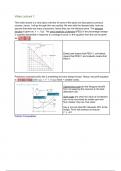
function is given as: 𝑃 = 𝑓(𝑄). The price elasticity of demand (PED) is the percentage change
in quantity demanded in response to a change in price. In the equation form this can be given
𝑑𝑄 𝑃
as: ϵ𝐷 = 𝑑𝑃
· 𝑄
.


Elastic part means that PED>1, unit elastic
means that PED=1 and inelastic means that
PED<1.


Producers maximize profit, this is something we have always known. Hence, the profit equation
is: π = 𝑝𝑞 − 𝐶(𝑞) and 𝐶(𝑞) = 𝐹 + 𝑉𝐶(𝑞) (fixed + variable costs).


Opportunity costs are the foregone benefit
from not applying the resource in the best
alternative use.

Sunk costs are when the value of investment
can not be recovered by resale upon exit
from market, they are ‘lost costs’.

Key is to know that MC intersects ATC at the
trough. Firms will produce as long as
𝑃 ≥ 𝐴𝑉𝐶
Perfect Competition:

, Assumptions in perfect competition:
(1) Many small buyers and sellers
(2) Perfectly informed
(3) Standardized Product
(4) Firms = price-takers.


Long run supply is at 𝑃𝐿𝑅, because firms
cannot affect prices.


Firms produce at MC=MR, hence at long run they produce at MC=P, since MR=P in the long
run. If MC>p, output decreases, if MC<P then output increases (as long as MC>AVC) and if
MC<AVC, the firm shuts down. This is because the firm continues making more and more
losses with every good sold, so it is not worth it to keep producing. In the long run, profits are
zero as there are no barriers to entry, so firms join or leave until profit becomes 0. Hence, in the
long run MC=P so vertical supply curve! Perfect competition is not realistic, but we use it as a
benchmark case, because it is efficient.

Monopoly:
Big barriers to entry so entry is not possible. Examples could be patents, natural monopolies,
etc. Monopoly also produces at MC=MR, to maximize its profits. MR intersects the x-axis
halfway as demand curve does, it is twice as steep!
Just know the graph, it is quite easy to
answer questions once you draw it out!

Monopolists earn profits, consumers lose
surplus that they would’ve had in a perfectly
competitive market, the loss in total surplus is
the DWL => Total Surplus (comp) - Total
Surplus (monopoly).


Monopoly Surpluses Perfect Competition Surpluses


Market Performance:

,Welfare is a big ting, for the formula: 𝑊 = π + 𝐶𝑆, hence, we can prove that monopoly always
has less welfare because: π𝑀 + 𝐶𝑆𝑀 < π𝐶 + 𝐶𝑆𝐶. We could also have weights, perhaps people
are happier than firms for an extra unit of surplus, hence; 𝑊 = θ1π + θ2𝐶𝑆, with θ1, θ2 ≥ 0. The
size of these parameters are a normative question!
Regulated Monopoly


This basically means a price ceiling, hence
the monopoly can not go above this price.
This reduces the DWL as seen in the graph
to the left.


𝑝−𝑀𝐶
Market power = ability to raise P above a perfectly competitive market. Lerner index: 𝑝
, this
is the ability to raise prices above MC as a percentage of the price, we can also set this as:
𝑝−𝑀𝐶 1 1
𝑝
= |ε|
(see instruction lecture 1). Monopolist: MR=MC and 𝑀𝑅 = 𝑝[1 − ε
] so with a low
PED, much more scope to raise price above MC, as opposed to a high PED.

𝑝−𝑀𝐶 𝑠
When there are several firms in the market, the lerner index is set as the following: 𝑝
= |ε|
where s is the market share

Market Concentration:
(1) # of firms?
(a) But this doesn't look at shares, what if 1 huge firm and 100 small firms?
(2) Concentration Ratio:
(a) =Market share of x largest firms in the industry, where market share means % of
total quantity produced
(b) Problem: Does not take inequality in market shares into account. E.G. two firms
have 50% concentration ratio, both 25% or one is 49% and the other 1%?
(3) Good Measure: Herfindahl index:
2 2
(a) H = sum of square of market shares =𝑆1 + ... + 𝑆𝑛
𝑞𝑖
(i) Where 𝑆𝑖 =
∑𝑞𝑖

This takes into account the # of firms in the industry, inequality of market shares and lies
between 0 (perfect competition) and 1 (monopoly).

, Video Lecture 2:
This lecture looks at price discrimination. It is important to remember that price discrimination
can only happen if firms have some degree of market power. So why price discriminate?
=> Lets the firm transfer consumer surplus to itself.
=> Welfare effects
=> May worsen market performance so this is a concern for public policy.
In order to discriminate, firms need to be able to have info about consumers’ WTP. Indirect info
= good too. There are poor and rich consumers, quality-conscious and non-quality conscious
consumers and much more. Lastly, it is also important to know that for some forms, arbitrage is
impossible. An example would be an airline ticket, or that there are too high transport costs to
resell.

There is Pigou’s approach on price discrimination, which looks at first-degree, second-degree
and third degree, however, we will more focus on the more modern approach. The first and third
degree are the same, but the second degree differs a little bit (also the names are different).

Types of Price Discrimination - Modern Approach:
Perfect Price Prices equal maximal WTP of consumers.
Discrimination

Self Selection Price and product structures devised by sellers that include
consumers to sort themselves into groups with different reservation
prices.

Selection by Indicators Consumers divided into groups (with each a different price
elasticity of demand), each group supplied at different profit
maximizing prices (e.g. senior and student discounts).


Perfect Price Discrimination:
Req: (1) Monopolist has perfect info about demand, ie, the monopolist knows WTP of
each consumer.
(2) arbitrage is not possible.

Voordelen van het kopen van samenvattingen bij Stuvia op een rij:

Verzekerd van kwaliteit door reviews

Verzekerd van kwaliteit door reviews

Stuvia-klanten hebben meer dan 700.000 samenvattingen beoordeeld. Zo weet je zeker dat je de beste documenten koopt!

Snel en makkelijk kopen

Snel en makkelijk kopen

Je betaalt supersnel en eenmalig met iDeal, creditcard of Stuvia-tegoed voor de samenvatting. Zonder lidmaatschap.

Focus op de essentie

Focus op de essentie

Samenvattingen worden geschreven voor en door anderen. Daarom zijn de samenvattingen altijd betrouwbaar en actueel. Zo kom je snel tot de kern!

Veelgestelde vragen

Wat krijg ik als ik dit document koop?

Je krijgt een PDF, die direct beschikbaar is na je aankoop. Het gekochte document is altijd, overal en oneindig toegankelijk via je profiel.

Tevredenheidsgarantie: hoe werkt dat?

Onze tevredenheidsgarantie zorgt ervoor dat je altijd een studiedocument vindt dat goed bij je past. Je vult een formulier in en onze klantenservice regelt de rest.

Van wie koop ik deze samenvatting?

Stuvia is een marktplaats, je koop dit document dus niet van ons, maar van verkoper mathieuvandevel. Stuvia faciliteert de betaling aan de verkoper.

Zit ik meteen vast aan een abonnement?

Nee, je koopt alleen deze samenvatting voor €7,96. Je zit daarna nergens aan vast.

Is Stuvia te vertrouwen?

4,6 sterren op Google & Trustpilot (+1000 reviews)

Afgelopen 30 dagen zijn er 62774 samenvattingen verkocht

Opgericht in 2010, al 15 jaar dé plek om samenvattingen te kopen

Start met verkopen
€7,96  1x  verkocht
  • (0)
In winkelwagen
Toegevoegd