Summary Statistics
Week 1
Statistics is the art and science of collecting, analysing, presenting, and interpreting data and
providing information to support decision-making. The modern ‘synonym’ is data science.
Terminology:
- Database, data set: all the relevant data to the topic.
- Columns: variables.
- Rows: observations, elements, cases, subjects.
- Each cell: measurement, data point.
Types of variables: level of measurement
- Qualitative data:
1. Nominal data: categories (no ordering or direction).
2. Ordinal data: ordered categories (rankings, order, or scaling).
- Quantitative data:
3. Interval data: differences between measurements, but no true zero.
4. Ratio data: differences between measurements, true zero does exist.
Types of data sets:
- Cross-sectional data: a survey of cases, all measured at one period of time, e.g. survey
conducted among customers.
- Time-series data: variables measured over time, e.g. various stock prices.
- Panel data: a combination of both: multiple cases, same variables measured at multiple
time points, e.g. consumer panel reporting purchase behaviour. This type is preferred.
Statistics is a way to get information from data.
A population is the group of all items/cases of interest. One has to conclude this group. A
sample is a group of items/cases drawn from the population. One applies statistical analysis
on the data from a sample.
Primary data is collected directly from the first-hand experience. This is the information that
you gather for the purpose of a particular research project.
Secondary data is the data that has been collected already for another purpose. The data is
collected by someone else instead of the researcher self.
,Symbols:
à → average
σ2 → standard deviation
S2 → estimated standard deviation
µ → mean
Categorical variables: tables
- Frequency distribution;
- Shown in a table;
- Absolute and relative frequency;
- Cumulative frequencies;
- Not too many categories. Otherwise: combine categories;
- Small categories could be combined in ‘other’.
Categorical variables: figures
- Often in a bar chart;
- Horizontal or vertical;
- With or without numbers (frequencies) added;
- Pie chart is more difficult to interpret. Use it only for categorical variables where the
percentage is relevant.
The valid percent differs from the percent when data is missing. This would also add another
category.
Numeric variables:
- Again, the frequency distribution is shown in a table.
- Absolute and relative frequency.
- Cumulative frequencies (more relevant here).
- However, often there are too many categories, so recording is needed (ages into age
categories).
- Not too many of too few groups: between 5 and 10 groups.
- If possible: equal distance between thresholds.
- Alternatively, aim at groups of similar size.
, Start data analysis of each project with descriptive statistics.
Get an overview of what is in the data.
Key characteristics of a distribution:
- Measures of central tendency (location): how high or
low are the values.
o Mode: most frequent one. Value of the variable
with the highest frequency in the database. The
only measure of central tendency for nominal
variables.
o Median: middle one. Middle observations if all
cases are ranked from low to high. To be used for ordinal and higher measurement
levels.
o Mean: average. To be used for interval and ratio variables only.
- Measures of variability: how much difference is there between observation.
o Minimum and maximum: to be used for ordinal and higher measurement levels.
o Range: difference between lowest and highest. Values observed in the data: min-
max. Only for variables with interval or ratio measurement levels.
o Interquartile range: the difference between the third and first quartile, so the middle
50% of the data, from observation 25% until 75%.
o Standard deviation: the amount of variation of a random variable expected about
its mean. Only for variables with interval or ratio measurement levels.
1. Population standard deviation:
∑(xi − μ)2
σ=√
n
2. Sample standard deviation:
∑(𝑥𝑖 − 𝑥̅ )2
𝑠=√
𝑛−1
x → each value in the data
μ → mean population
𝑥̅ → mean sample
n → number of data points
∑ → sum
o Variance (square of deviation): expected value of the squared deviation from the
mean of a random variable. Only for variables with interval or ratio measurement
levels.
The coefficient of variation is a relative measure of variability. How much variation there is in
the sample, relative to the mean of the variable. Comparable across variables that differ in
𝜎
scaling/size (thus, in average/mean). 𝐶𝑣(%) = 𝜇 ⋅ 100
Additional characteristics of distributions:
- Shape of the distribution: symmetric (skewness = 0) or skewed (right or left). Only
relevant for variables with interval or ratio measurement levels.


