Transport & Supply Chain
HC 1
EU transport policy; aim is efficient, safe and sustainable transport policies to create competitive industry
with jobs & prosperity
Economics of Demand → Derive demand by maximizing utility
Effective demand; amount that consumers are willing and able to buy a product at a given price.
Derived demand; products are wanted, not of their value, but because they allow consumers to satisfy other
demands (benzine)
What can we do with a demand function? > Firms: estimate demand functions to predict demand
> Policy maker: determine welfare
> Willingness-To-Pay: what does the client want to pay?
Assumptions: consumer decides based on given information (rational) and self interest to maximize utility U.
Indifference curve: combination of two goods or qualities (Q1 & Q2) that gives consumer
same satisfaction/utility.
Inverse demand; p1 = p2*ΔQ2/ ΔQ1 —> p1 is maximum price we are willing to pay so that our utility is
maximized for unit p1.Benefit derived from Q1 is used as a measure of welfare. It measures how much of Q2
is given up for Q1, given that utility is maximized.
- Marginal benefit determines slope
- Point D is optimum → slope budget curve = slope indifference curve p1/p2 = ΔQ2/ΔQ1
Consumer decides quantity of Q1 & Q2 depending on his budget constraint:
Y= p1*Q1+p2*Q2
Determinants demand (increase in price leads to lower quantity):
- Price of substitutes
- Price of complementary goods
- Income
- Population; higher population —> higher demand
- Bureaucracy
- Security; when e.g. shipping diamonds
- Popularity/image; media image
- Speed; delivery time
- Reliability; how reliable is delivery?
Elasticity of demand= responsiveness of demand to a change in a factor (bv. price), measured in %
Price elasticity (ped)= (% change output) / (% change price)= (∆Q/Q) / (∆P/P) = (∆Q/∆P) * (P/Q)
∆X = %∆X = (Xnew -Xold)/Xold *100
Point elasticity; measured in a point price elasticity: (∂Q/∂P)*(P/Q) → ∆P=∂Q/∂P Reverse demand is
Price elasticity of -1.15 means, demand increases with 1.15% if price increases with 1% lineair at ped=1
Inelastic demand: -1 < ped < 0
Elastic demand: ped < -1
,Price elasticity is influenced by;
- Proportion of consumer expenditure
- Addictiveness
- Level of necessity
- Time scale; (more time, more time for substitute, the more elastic
demand will be)
- Availability of substitutes
Elasticity cannot be controlled because you can’t control consumers
budget, you can make it more addictive or make goods appear more
necessary, time scale → often updates to appear to be better (apple).
And you can try to get rid of substitutes.
Welfare
Inverse demand curve gives willingness-to-pay. Area under demand curve measures total benefit or total
surplus (welfare)
HC 2 Cost functions Q=f(P,Y,t) Demand Q is a
function of price P, income Y and
time trend t.(assumes a causal
PS relation between variables).
Q=α*P+β*Y+γ*t OR
CS lnQ=α*lnP+β*lnY+γ*t
HC2
Production factors need to be chosen so that costs are minimized (transport; land; fuel, labor; driver,
capital; truck, entrepreneurship)
> Produce output Q (Q=δL^α*K^β: Cobb-Douglas production function
> Labour(L) at price w, capital(K) at price r, α and β are weights for L and K in the production function
> Minimize: C=w*L+r*K
> Cost function C=C(Q,r,k): minimum cost of producing Q given input prices, using optimal levels of (K,L).
Cost minimization: slope iso-cost = slope isoquant r/w=ΔL/ΔK
Cost function requirements: increasing Q, non-decreasing in input
prices (w, r), → C(Q ,x*w,x*r)=x*C(Q ,w,r)
Application of cost function (implicitly) assumes cost minimization!
Cost function; gives minimum cost of producing a given output level → Assumes cost minimization!
> Interesting because it determines (minimum) cost in welfare analysis, economies of scale, benchmarking.
Fixed costs; cost are the same, irrespective of output produced (rent, insurance)
Variable costs; cost that change as level op output changes (fuel) LET OP; outsourcing transforms fixed into
variable costs.
Marginal costs: change in TC due to a unit change in output (additional TC incurred by producing extra
unit) MC= ∂TC/∂Q
Sunk cost= expenditure that a producer has to make in order to enter a market that is unrecoverable on exit
from the market
, Cost function: C(Q,w,r)
Elasticity of cost with respect to output: >(∂TC/∂Q)*Q /TC = (∂TC/∂Q)/(TC/Q) = MC/AC
>MC < AC: economies of scale or increasing returns
>MC > AC: diseconomies of scale or decreasing returns
>MC = AC: No economies of scale (constant returns to scale)
Economies of Scale; average costs decrease as output increases
- Technical economies of scale (aircraft size)
- Managerial economies of scale (good reputation producers attract efficient but more expensive
management)
- Marketing economies of scale (large producers can negotiate favorable contracts with suppliers)
- Financial economies of scale (large producers perceived to have lower risks)
Diseconomies of Scale:
- Red tape (paper work and coordination effort increases with size of producer)
- Communication problems (chain of command becomes longer as producer grows)
Economies of density(scope); Average costs are reduced when output is increased by using existing fixed
capital (density increases) - Savings gained by producing two or more distinct goods, when cost of doing so
is less than producing each separately
> (∂C/∂Q)*Q/C = MC/AC
Focus network; economies of scale → RTD = 1/εQ = 1/[(∂C/∂Q)*Q/C] = AC/MC (measured in passengers)
If RTD >1 when we increase passenger number in our network, average cost per passenger decreases
Cobb-Douglas; Output parameter in the cost function is the elasticity (ε) of cost with
respect to output.
>
>
Translog parameter ε; >
Problem with Cobb-Douglas: scale elasticity (ε) is the same for every firm or output size.
Labour= total labour costs / number of employees (high if there are many CEO’s)
Equipment= equipment costs / net value of airport property(=value-depreciation-sales of asset)
Residual(operational cost – labour – equipment) / net value of airport property
Assume Schiphol and Lelystad have similar elasticities (0.45 and 0.27). Cost impact of moving flights to
Ley? If cost margin changes, elasticity will change. IF there are scale economies at schiphol. with the
strategy of moving flights to smaller airports will change profit margin. Revenue of schiphol will decrease.
That’s why you need to do a Cost function estimation
Cost function gives total cost as a function of output and prices of all inputs. It assumes that firm works
as efficient as possible. Conditions: 1. Total cost increases with an output.
2. Total cost does not decrease with a price.
3. All inputs are included
Cost function estimation important in transport; Scale effect= as price of one input changes, there is a
resulting change in total volume of output that producer would like to sell and so employment will change as
well. Transport has most economies of scale
HC 3 Market structures
> Revenue; Consumers; inverse demand gives willingness to pay
Producers; cannot set price higher than inverse demand at given Q
Marginal revenue; change in revenue due to change in output (additional revenues from next
unit sold)
Revenue= Price*Quantity
MR = ∂R/∂Q (derived revenue) → twice as steep as linear inverse demand function


