Alba Kalayci-Nicault
SNR: 2036559
Microeconomics: Markets and Games
Midterm: 11 March (15:00 – 17:00) 25% of course grade
End term: 4 April 75% of course grade
- Covers everything, but second part of the course will have more weight (over 50% of
the questions)
- 35 questions in 2 hours
- Know the math!!
Week 1: Basic Concepts
KC1: Production Function
- A firm’s success and ability to grow partly depends on its pricing and production
decisions
- Firm transforms inputs into outputs
- Two types of inputs:
o Fixed input: cannot be changed in the short run, fixed for a period (e.g., land)
o Variable input: can be changed at any time (e.g., labor, intermediary good)
o Short v long run: in the long run all inputs can be adjusted
o For now, we focus on the short run (i.e., one input is fixed)
- Production function: relationship between quantity of input and quantity of output
(for a given amount of fixed input)
o Two characteristics:
o Slope is positive: more input generates more output
o Slope gets flatter: contribution of last unit of input to output gets smaller
- Marginal product of input: change in output generated by adding one unit of input,
given an amount of the other input (marginal analysis)
o Downward-sloping
o Linear
o Typical pattern: marginal product of input is always positive but becomes
smaller with more input used
,Alba Kalayci-Nicault
SNR: 2036559
- But marginal product can even become negative at some point, e.g., if firm hires too
many employees who distract each other
Describing production: Economies of scale
- A firm’s costs depend on its scale of production and the type of production
technology it has
- Large firms can be more profitable than small firms because of technological and/or
cost advantages, we say that production exhibits:
- Increasing returns to scale (economies of scale)
o If inputs increase by a given proportion, and production increases more than
proportionally
- Constant returns to scale
o If inputs increase by a given proportion, and production increases by the same
proportion
- Decreasing returns to scale (diseconomies of scale)
o If inputs increase by a given proportion, and production increases less than
proportionally
Economies of Scale: Examples
- Economies of scale includes:
- Cost advantages – large firms can purchase inputs on more favorable terms, because
they have greater bargaining power when negotiated with suppliers
- Demand advantages – network effects (value of output rises with number of uses
(e.g., software application))
- However, large firms can also suffer from diseconomies of scale, e.g., additional
layers of bureaucracy due to too many employees
KC2: Cost Function
- To make pricing and production decisions, managers need to know the costs of
production
- Cost function: shows how total production costs vary with quantity produced
- Two characteristics:
o Slope is positive: the cost increases with the quantity of output
o Slope gets steeper: more input must be used to produce each additional unit of
output
,Alba Kalayci-Nicault
SNR: 2036559
Cost Function
- Total Cost (TC) = Variable cost (VC) + Fixed cost (FC)
- Fixed cost (FC): cost of fixed input (e.g., rent per month for the location of restaurant
or production site, rent for land, etc.)
- FC does not depend on the quantity of output produced in the short run
- Variable cost (VC): costs such as salary of workers, electricity, cost of intermediary
goods, etc.
- VC increases with the quantity of output produced: more output requires more units
of variable input
Average cost
- Average cost per unit of output produced
- Calculated as the slope of the ray from the origin to a given point on the cost function
- In this example, average cost decrease at first (economies of scale), but then increase
(e.g., overtime, machine breakdown)
- Average total cost (ATC): TC (total cost) / Q (output)
- TC = 20 + 50Q
- ATC = (20 + 50Q) / Q = 20/Q + 50
, Alba Kalayci-Nicault
SNR: 2036559
Marginal cost
- The effect of total cost of producing one additional unit of output
- Calculated as the slope of the cost function at a given point (draw tangent at that
point)
- In this example, marginal costs increase with production
- TC = 20 + 50Q
- MC (derivative of total cost) = dTC / dQ
o MC = 50 because derivative of 20 is 0 and derivative of 50Q is 50
Relationship between MC and AC
- The following statements are always true:
- If AC > MC: AC is decreasing
- If AC < MC: AC is increasing
- The MC curve always intersects the AC at its lowest point
KC3: Profit Maximization & Gains from Trade
Demand Curve
- To make pricing and production decisions, managers also need to know the demand
for the firm’s product
- Demand curve shows the quantity that consumers will buy at each price
- In theory, firms can estimate the demand curve for their product by surveying many
consumers
Isoprofit curve
- (Economic) Profit = Total revenue – Total costs