Test Description Variable type Hypotheses Conditions Remark Example
Test whether the larger part of
Test whether a population Test for normality the US population is in favour of
One sample 1 Quantitative H0: X =1000 Random and normally
mean is significantly different (Lilliefors) and the health insurance program
t-test variable H1: X ≠ 1000 distributed or n >30
from some hypothesized value. skewness than opposed (1 favour, 0
neutral, -1 opposed)
X1 = rating 1 (before the campaign), X2
Estimate differences between 2 2 Quantitative Test for normality
Paired = rating 2 (after the campaign) Random and normally Test whether training has a
locations. For each item there is variables (e.g. (Lilliefors) and
samples H0: X1 = X2 (or X1 – X2 = 0) distributed or n >30 positive effect on productivity
a pair of observations. before and after) skewness
H1: X1 ≠ X2 (or X1 – X2 ≠ 0)
Levene’s test: if
Estimate differences between 2 Random & independent
2 Independent p > 0,10 H0 is not Estimate the productivity
Independen locations. For each sample H0: X1 = X2 (or X1 – X2 = 0) samples, normally
quantitative rejected and difference between full- and
t samples there is an independent H1: X1 ≠ X2 (or X1 – X2 ≠ 0) distributed or n >29 and
variables equal variances part timers
sample. not (too) skewed
assumed
H0 population correlation = 0
Correlation Test the linear relation between 2 Quantitative Weak, moderate, Measure linear correlation
H1: population correlation ≠ 0
coefficient variables variables strong [-1, 1] between productivity and age
H0: the two variables are independent,
Test relation. Test statistic that Is there a relationship between
(variables are not associated) Random, Ej > 5, normally
measures differences between 2 Categorical age (18-20, 21-23, 24-26 and
Chi-squared H1: the variables are dependent distributed or n >29 and
O and E frequencies in a cross variables older) and attitude (bad,
(variables are not associated) not (too) skewed
table neutral, good)?
Describe relation. Measures the Measure the relation between
2 Nominal Weak, moderate,
Cramer’s V strength of the association - - gender (male, female and male)
variables strong [0, 1]
between variables and plastic surgery
Measure the relation between
Describe relation. Measures the job satisfaction (satisfied,
Kendall’s 2 Ordinal Weak, moderate,
strength of the association - r=c neutral) not satisfied and
tau-b variables strong [-1, 1]
between variables commitment (committed,
neutral, not committed)
Measure the relation between
Describe relation. Measures the
Kendall’s 2 Ordinal Weak, moderate, age (18-20, 21-23, 24-26 and
strength of the association - r≠c
tau-c variables strong [-1, 1] older) and attitude (bad,
between variables
neutral, good)
H0: PMx = 20 transform with Y = ln(X)
The distribution of waiting time
transformation is a replacement H0: PMy = ln(20) = 2,996 You use
of clients is skewed to the right.
Transfor- H0: μy = 50, transform with Y = √X. Random and normally transformations if
that changes the shape of a Test whether efforts to reduce
mation distributed or n >30 the distribution is
distribution or relationship. √X = 50, so X= 50kwadraat H0: PMx the waiting times are reduced
too skewed.
successfully.
= 2500