INT9: H16: Understanding Consumer Behavior
Solow growth model shows that the saving rate is a key determinant of the steady-state capital stock
and therefore of the level of economic well-being. It measures how much income the present
generation is putting aside, so not consuming, for the future. Consumption is important as it makes
up 2/3 of GDP and causes important fluctuations.
John Keynes’ consumption function
- The marginal propensity to consume, amount consumed of 1 additional dollar of income, is
always between 0 and 1;
o Men usually increase consumption as income rises, but they can’t spend more than
they earn.
- The average propensity to consume falls, which is the ratio of consumption to income, when
income increases;
- Keynes believes that income is the key determinant of consumption and the interest rate is
unimportant.
o Other economists disagreed with this statement of the interest rate, but Keynes
thought that the short-term influence of the interest rate on individual spending is
secondary and relatively unimportant.
C = consumption, Y = disposable income, C(bar) = constant, c = marginal propensity to consume
(between 0 and 1). C(bar) determines the vertical axis intercept, c determines the slope.
Keynes’ second property is satisfied as C(bar) falls as Y rises, which results in C/Y decreasing. The
equation below also satisfies his tried property as the interest rate isn’t included in the equation.
Researchers found that households with higher incomes consumed more, MPC > 0. Higher income
households saved more, MPC < 1. Higher-income households saved a large percentage of their
income, showing that APC decreases as income rises. So Keynes’ views were confirmed.
,Two abnormalities did occur w.r.t the average propensity to consume falls as income rises:
1. After WW2, according to Keynes, households would consume less when income increases, so
economists feared that there might not be sufficient profitable investment projects to absorb
all these savings. In turn, this low consumption would lead to little demand for goods,
resulting in post-wartime depression. So Keynesian economists predicted secular stagnation
– a long depression of indefinite duration – unless the government would apply fiscal policy
to expand aggregate demand. Fortunately, after WW2 Keynes’ theory that APC would falls as
income rose did not hold.
2. The economist Kuznets’ data showed that the ratio
of consumption to income was stable for decades,
contrasting Keynes’ theory that APC decreases as
income rises.
Evidence shows that the Keynesian consumption function
works well for short time-series and household data, but it
doesn’t hold in the long time-series as the APC remains
constant.
Irving Fisher and Intertemporal choice
Consumers face limits on how much they can consume, a budget constraint. When deciding how
much they consume today and how much they save for the future, they face an intertemporal
budget constraint.
There are two periods, C1 and C2, C1 represents consumption in customer’s youth, C2 in old age.
They earn income Y1 in C1 and Y2 in C2. S = Savings. r = interest rate.
S = Y1 – C1
In the second period, C2 equals the accumulated saving of period 1 including interest, plus second-
period income:
C2 = (1 + r)S + Y2
The variable S can represent saving or borrowing. If consumption in period 1 is less than income, it is
saving, if consumption is more than income, it represents borrowing. We combine the two functions
to create the consumer’s budget constraint:
C2 = (1 + r)(Y1 – C1) + Y2
We can simplify this to create the intertemporal budget constraint:
->
The consumer’s budget constraint is easily explained. If the interest rate is 0, then total consumption
of the two periods equals total income in those periods. If r > 0 then future consumption and income
is discounted by (1 + r). This discounting arises from interest earned on savings. Similarly as future
consumption is paid for out of savings that have earned interests, future consumptions costs less in
comparison to current consumption (namely, 1/(1+r)).
, In point A, consumption
equals income in both
periods (C1=Y1, C2=Y2).
In point B, C1=0, all income
is saved so that
C2=(1+r)Y1 + Y2.
In point C, everything is
consumed in period 1
(C2=0), so that
C1=Y1+Y2/(1+r)
Customer preferences
Indifference curves show the
combination of first and second-period
consumption that makes consumers
equally happy. The consumers is
equally content with point X, Y, W, but
prefers point Z as a higher curve is
better.
The slope at any point shows how much
second-period consumption is required
to compensate for a 1-unit reduction in
first-period consumption. The slope is
the marginal rate of substitution, so it showcases the rate at which one is willing to substitute second
period consumption for first-period consumption. When first-period consumption is high and second-
period consumption is low, as at point W, the marginal rate of substitution is low.
Optimization
A consumer is satisfied the most when the budget constraint is tangent
to the highest indifference. The slope of the indifference curve is the
MRS (marginal rate of substitution). The slope of the budget line is
(1+r). So point O -> MRS = 1+r
An increase in income leads to a shift of the budget constraint to the
right. If a consumer wants more of a good when his income rises, it is a
normal good.
Consumption smoothing is the spreading of consumption over periods. Key is that consumption
depends on the present value of current and future income:
Keynes: A person’s current consumption depends on his current income
Fisher: Consumption is based on income that one expects over his entire lifetime.


