Formuleblad Data-Analyse | T1 & T2-Stof By Rico Keizer σ X ,Y
ρ=ρ X , Y =
*Red-Underlined Text Refers To SPSS Matters* σ X σY
o −1 ≤ ρ ≤ 1
T1-Stof:
sX , Y
Chapter 5 | Pairs Of Variables r =r X , Y =
sX sY
Descriptive Statistics: o −1 ≤r ≤ 1
SPSS > Analyze > Descriptive Statistics: The Correlation shows the degree of linear
relationship.
+1 : All plotted dots lie on an increasing line.
-1 : All plotted dots lie on a decreasing line.
0 : All plotted dots are uncorrelated.
Average: ( μ∨ x) SPSS > Analyze > Correlate > Bivariate:
N
1
μ= ∑x
N i=1 i
n
1
x= ∑x
n i=1 i
Variance: (σ 2∨s 2)
N
21
σ = ∑ ( x i−μ x )
N i=1
n
1
s2= ∑ ( x −x )
n−1 i=1 i
Covariance: (σ x , y ∨s x , y )
N
1
σ x , y = ∑ ( x i−μ x ) ( y i−μ y ) Linear Transformation Rules:
N i=1
n
V =a+bX ∧W =c+ dY
1
s x, y = ∑ ( x −x ) ( y i− y )
n−1 i=1 i Average:
N μv =a+b μ x ∨v=a+ b x
1
s x, y = ∑x y− n xy
n−1 i=1 i i n−1 Variance:
The Covariance shows the strength of a relationship. 2 2 2 2 2 2
σ v =b σ x ∨s v =b s x
Use a graph to check what kind of relationship.
SPSS > Graphs > Chart Builder > Scatterplot Standard Deviation:
σ v =|b|σ x ∨s x =¿ b∨s x
Covariance:
σ v ,w =bd σ x , y ∨s v , w =bd s x , y
Correlation Coefficient:
Quadrants I and III suggest σ x , y ∨s x , y >1 bd >0 → ρv ,w =ρx , y ∨r v, w =r x , y
Quadrants II and IV suggest σ x , y ∨s x , y <1 bd <0 → ρv ,w =−ρ x, y ∨r v ,w =−r x , y
Correlation: ( ρ∨r )
, Manually Making A Descriptive Statistics Table:
Assumptions Of A Simple Linear Regression Model
This table can be used manually to find out most of And Residual Analysis:
the descriptive statistics. Linearity:
Chapter 19 | Simple Linear Regression The mean of ε is equal to zero: E ( ε|x ) =0
General Setting: Visual Check:
A population with k+1 variables,
Dependent Variable Y
Independent Variables X 1 , … , X k
Objective:
How Y depends on X 1 , … , X k
Learn about the strength of that relationship
Predict Y for known values of X 1 , … , X k SPSS > Create a scatterplot of Unstandardized
The Simple Linear Regression Model: Residual by X. Check whether the spread under and
above the 0-line is equal at all points. If so, linearity is
Population Form: Y = β0 + β 1 x+ ε satisfied.
^ =B + B x+ e
Sample Form: Y Homoskedasticity:
0 1
2
Regression Coefficients: ( β 0 , β 1∨B0 , B 1) The variation of ε stays the same: V ( ε|x )=σ ε
β 0=μ y −β 1 μ x Visual Check:
σ x,y
β 1=
σ 2x
B0= ^y −B 1 x
sx , y
B1= 2
sx
Regression Lines: (Y ∨Y^ )
SPSS > Create a scatterplot of Unstandardized
y=β 0 + β 1 x Residual by ^y . Check whether the vertical spread
changes from one point at ^y to another. If this isn’t
^y =b0 +b1 x
the case, homoskedasticity is satisfied.
Residuals: Independence:
e n= y n −^y n All pairs ( x n , y n ) are a random sample, thus ε n are
n independent too.
o ∑ ei=0 Visual Check:
i=1
Residuals show the estimated errors for all
observations i .


