Symbols:
μ = Population mean
μ̂ = Estimated population mean
ȳ = Sample mean
y = Single outcome of one thingie
σ = Standard deviation of population
σ2 = Variance of population
σ̂ = Estimated std deviation of population
σ̂2 = Estimated Variance of population
s = Std deviation of sample
s2 = Variance of sample
se = Std error of sample
e = Error (half the confidence interval)
k = Number of explanatory variables
N = Grand sample size
n = Treatment sample size
Formulas:
ȳ = μ ̂
2
(yi − ȳ)2
s =
n−1
σ̂2 = s 2
s= s2
σ = σ̂2
2
(n1 − 1) * s12 + (n2 − 1) * s22
s =
n1 + n2 − 2
σ
se =
n
Sample Size Calculations:
For one sample:
Based on the width of the confidence interval for μ:
(za/2)2 * σ 2
n= In which E = required or expected error margin (CI divided by 2)
E2
Based on hypothesis testing for μ:
(za + zβ )2
n= In which Δ = μ1 − μ0el (or smallest difference in which you have an
(Δ/σ 2)
1
, interest), and β = 1 − power , while Z comes from Critical Z table
This formula is for one sided hypothesis, for two sided hypothesis
its za/2.
For paired data:
Formulas are exactly the same, but with σ instead of regular σ
d
For two sample t-test:
Everything stays the same (including regular sigma) but with a 2 in front of the formula. Note that
the n you’re calculating is for 1 sample, and has to be multiplied by two again if you would like to
have the entire sample.
For single binary data:
Exactly same as first formula, where σ 2 = π ̂ (1 − π)̂
One Sample T Test:
( ȳ − H0) ȳ − H0
TS: t = (when σ is unknown. If sigma is known: z =
s2 σ/ n
N
t ~ t (df = n-1) or z ~ z(0,1)
SPSS Gives 2-sided P, so P/2 for one sided hypotheses
CI: ȳ ± ta/2,df * s / n or ȳ ± za/2,df * σ / n
Paired T Test:
Basically a one-sample t-test on the differences and its standard deviation.
d¯ − D0
TS: t = CI: d¯ ± ta/2,df * sd / n
sd2
n
Independent Samples T Test:
Equal variances
( ȳ1 − ȳ2) − D0 ( ȳ − ȳ2) − D0 1 1
TS: t = = 1 CI: ȳ1 − ȳ2 ± ta/2,df sp +
se(y1 − y2) 1 1 n1 n2
sp +
n1 n2
In which sp = s2
Unequal variances
2


