Samenvatting

Summary Marketing Strategy Research | MSc Marketing Management | RSM - Erasmus University

0 keer verkocht

Instelling
Erasmus Universiteit Rotterdam (EUR)

Complete summary of all the lectures, tutorials and cases of the course Marketing Strategy Research given by Xi Chen in the master program Marketing Management. Good luck with studying!

[Meer zien]

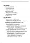
Voorbeeld 2 van de 7 pagina's

Bekijk voorbeeld

Geupload op 4 januari 2024
Aantal pagina's 7
Geschreven in 2023/2024
Type Samenvatting

marketing management
master
xi chen
rstudio
marketing strategy research
summary
samenvatting

Volgen

Daniquedhs Lid sinds 6 jaar 360 documenten verkocht

€5,99

In winkelwagen

Op verlanglijstje

100% tevredenheidsgarantie
Direct beschikbaar na je betaling
Lees online óf als PDF
Geen vaste maandelijkse kosten

SUMMARY MARKETING STRATEGY RESEARCH

WEEK 1 | INTRODUCTION
 Consumers  data  tools  strategy
 There are 9.932 analytical tools – this course covers 5
o Linear regression: market responses
o Conjoint analysis: new project design
o Bass model: new project diffusion
o Cluster analysis: segmentation
o Multi-dimensional scaling: positioning
 Principles of data-driven marketing
1. Any statistical analysis is to reduce information loss
2. Causation cannot be learned directly from data
3. Prediction does not care about statistical significance
4. Practical usefulness triumphs statistical criteria
 Case: pricing strategy for Jetstar
o Formulate strategies based on analytical results

WEEK 2 | LINEAR REGRESSION
LECTURE
 What & why: intro to predictive modeling
o Market response model: how to predict market response
o E.g. Target knowing when someone is pregnant based on behavior
o Prediction machine: find functional relationship between input (data) and output (prediction)
o Linear regression = simplest form, straight line / : y = a + bx - with an intercept and b slope
 Terminologies: with a toy example, using price to predict sales - sales = a + b*price
o X: price = independent variable - input
o Y: sales = dependent variable - output
o Principle: any statistical analysis is to reduce information loss
 Prediction as close as possible to observations – choose line to minimize differences
 How: 5 steps to perform a linear regression
o Examining the data: make sure data is clean, check for correlation, multi-collinearity, etc.
 Multi-collinearity: VIF < 10 not an issue, VIF > 10 high collinearity
 High correlation indicates trouble, get biased and misleading estimated coefficients
 Use one variable in regression, transform correlated variables, collect more data
o Formulating the model: decide which variables to use as input: IV's, DV, and residual
 Translate conceptual model to a R formula
o Estimating the model: any statistical analysis to minimize information loss (residuals)
 Choose coefficients so differences (residuals) between actual & predicted are minimized
 Least squares criterion: minimize residual sum of squares (RSS)
o Validating the model: look at model's significance
 Naïve prediction: prediction with only intercepts, but no other IV's - assumption
 Null hypothesis using F statistics and check p-value in R output - significance
 R-squared: model fit or strength of association - % of variation in DV explained by model
 How good is the model for prediction? – validate the model
 Test significance of individual coefficient: H0, t-test, check p-value

, o Making predictions: use predict() function, a new data set and confidence interval
 Extending the use of linear regression
o Nominal variables: cannot directly put into a regression - need to be numeric
 Designate a variable as factor: R will do the rest – weather <- as.factor(weather)
o Dummy coding (binary variable, 0-1) - always baseline
 M-1 dummy variables, choose baseline: weather <- relevel (weather, ref=”sunny”)
o Interpretation of coefficients: we only know the difference between conditions
 When coefficient not significant: difference of baseline not significant: same level
 Risk control: assumptions in linear regression on residuals
o Normality - test using residuals in histogram or K-S test
o Equal variance - test using scatter plot or Y^ and residuals
 Obtain residuals and DV -> standardize both -> draw scatter plot x-as DV and y-as residue

TUTORIAL
 Step 1 checking the VIFS: vnames <- colnames(train)[2:5] & vif(vnames, train)
 Step 2 formulate model: Sales = β0 + β1IV1 + β2IV2 + β3IV3 + β4IV4 + е
 Step 3 estimate model: model <- lm(Sales ~ IV + IV + IV + IV, data = train) & summary(model)
 Step 4 validate model: check significance of overall model and coefficients
o Test H0: β1 = β2 = … = 0 & H0: βk = 0 | when p < 0.05 reject H0: predictive value
o Check R-squared = % variation explained by model – depends on environment (>90% sales)
 Step 5 make predictions: test <- set[76:100,] & str(test) & model2 <-predict(model, newdata = test)
o Model2 <- as.data.frame(model2) & model2$week <- 76:100 & ggplot
 Comparison: Repeat steps without IV Brand Equity and compare the two models
 Risk control: violation leads to biased estimation and bad prediction
o Normality assumption: KS test H0: The variable follows a normal distribution
 H0 should not be rejected, so KS test should NOT be significant p > 0.05
o Equal variance assumption: plot residuals and check if span/ranges are similar
 Categorical variables cannot go in regression: first transformed to factors – setting a baseline
o Interpretation is tricky: always relative to the baseline

CASE
 Product line cannibalization = older lines not selling anymore after introducing new ones
 Objective: to find possible cannibalization effects
o How introduction and sales of new styles influence sales of the previous line
 Causation ≠ correlation – causal structures can produce same correlation pattern
o Confounder variables: contaminates the causal effect
 add to regression as control variables to kill lurking variables
 Week as control variable - week 1 is baseline
 Simple running a regression gives you correlation: causation is difficult to get in practices

WEEK 3 | CONJOINT ANALYSIS
LECTURE
 To understand preferences = holy grail – voting, consumption, social life
 Product is combination of attributes & levels – e.g. decide product attributes of laptop
o Manager = chef, attributes = ingredients, conjoint analysis = recipe

Dit zijn jouw voordelen als je samenvattingen koopt bij Stuvia:

Bewezen kwaliteit door reviews

Studenten hebben al meer dan 850.000 samenvattingen beoordeeld. Zo weet jij zeker dat je de beste keuze maakt!

In een paar klikken geregeld

Geen gedoe — betaal gewoon eenmalig met iDeal, creditcard of je Stuvia-tegoed en je bent klaar. Geen abonnement nodig.

Direct to-the-point

Studenten maken samenvattingen voor studenten. Dat betekent: actuele inhoud waar jij écht wat aan hebt. Geen overbodige details!

Veelgestelde vragen

Wat krijg ik als ik dit document koop?

Je krijgt een PDF, die direct beschikbaar is na je aankoop. Het gekochte document is altijd, overal en oneindig toegankelijk via je profiel.

Tevredenheidsgarantie: hoe werkt dat?

Onze tevredenheidsgarantie zorgt ervoor dat je altijd een studiedocument vindt dat goed bij je past. Je vult een formulier in en onze klantenservice regelt de rest.

Van wie koop ik deze samenvatting?

Stuvia is een marktplaats, je koop dit document dus niet van ons, maar van verkoper Daniquedhs. Stuvia faciliteert de betaling aan de verkoper.

Zit ik meteen vast aan een abonnement?

Nee, je koopt alleen deze samenvatting voor €5,99. Je zit daarna nergens aan vast.

Is Stuvia te vertrouwen?

4,6 sterren op Google & Trustpilot (+1000 reviews)

Afgelopen 30 dagen zijn er 69411 samenvattingen verkocht

Opgericht in 2010, al 15 jaar dé plek om samenvattingen te kopen

Begin nu gratis

Samenvatting

Summary Marketing Strategy Research | MSc Marketing Management | RSM - Erasmus University

Document informatie

Onderwerpen

Geschreven voor

Verkoper

Ontvangen beoordelingen

Voorbeeld van de inhoud