statistics.
There are two alternative forms of the theorem, and both alternatives concern
drawing a finite samples size 𝑛 from a population with a known mean, μ, and a
known standard deviation, σ.
First alternative: Collect samples of size 𝑛 with a large enough 𝑛, calculate each
sample's mean, and create a histogram of those means, then the resulting histogram
will tend to have an approximate normal bell shape.
Second alternative: Collect samples of size 𝑛 that are large enough, calculate the
sum of each sample and create a histogram, then the resulting histogram will again
tend to have a normal bell shape.
In either case, it does not matter what the distribution of the original population is.
It’s important that the distributions of sample means and the sums tend to follow
the normal distribution.
The size of the sample, 𝑛, that is required in order to be large enough depends on
the original population from which the samples are drawn (the sample size should be
at least 30 or the data should come from a normal distribution).
If the original population is far from normal, then more observations are needed for
the sample means or sums to be normal. Sampling is done with replacement.
The Central Limit Theorem for Sample Means (Averages)
Suppose 𝑋 is a random variable with a distribution that may be known or unknown (it can
be any distribution). Using a subscript that matches the random variable, suppose
a. 𝜇𝑥 = the mean of 𝑋
b. 𝜎𝑥 = the standard deviation of 𝑋
If you draw random samples of size 𝑛, then as 𝑛 increases, the random variable 𝑋̅, which
consists of sample means, tends to be normally distributed and
The central limit theorem for sample means states that if you keep drawing larger and
larger samples and calculating their means, the sample means form their own normal
distribution (the sampling distribution).
The normal distribution has the same mean as the original distribution and a variance that
equals the original variance divided by the sample size. The variable 𝑛 is the number of
values that are averaged together, not the number of times the experiment is done.
1
, If you draw random samples of size 𝑛, the distribution of the random variable 𝑋̅,
which consists of sample means, is called the sampling distribution of the mean.
The sampling distribution of the mean approaches a normal distribution as 𝑛, the
sample size, increases.
The random variable 𝑋̅ has a different 𝑧 −score associated with it from that of the
random variable 𝑋.
The mean 𝑥̅ , is the value of 𝑋̅, in one sample.
Tips for using a statistical calculator to find the above:
2

