100% satisfaction guarantee Immediately available after payment Both online and in PDF No strings attached
logo-home
Summary Cheatsheets for Data Mining and Machine Learning courses R156,27   Add to cart

Summary

Summary Cheatsheets for Data Mining and Machine Learning courses

1 review
 123 views  12 purchases
  • Course
  • Institution

The file contains cheatsheet materials for two M.Sc. DSS core courses, Data Mining for Business & Gov. (880022-M-6) and Machine Learning (880083-M-6). Both cheatsheets have been tested on multiple mock exams as well as used successfully in the actual exams. Includes python codes for Machine Learni...

[Show more]
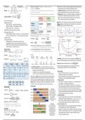
Preview 1 out of 4  pages

  • January 15, 2024
  • 4
  • 2023/2024
  • Summary

1  review

review-writer-avatar

By: franciscorau08 • 4 months ago

avatar-seller
Normalization Standardization Pr[outcome1 | evidence] = ∏ Pr[featurei = evidencei | outcome1] * • kNN: sensitive to outliers, the number of neighbors and the distance function.
Pr[outcome1] / Pr[evidence] The smaller the value of k, the more likely the model to overfit.
Pearson ∈ [-1, 1] Pr[evidence] is constant. Calculate the green part for both outcomes first • Stratification procedure: ensures that decision class distrib. of a given
and then obtain Pr[evidence]. sample is proportionally similar to decision class distrib. of whole pop.
#!∘ #∘" % NB assumes that features have the same importance and are independent. • Random search: explores a set of possible combinations. It might overlook
"#!" $ % good models but is faster and usually gets the job done. Can be used to
Chi-sq. association χ! = ∑*+() ∑&'() #
#!∘ #∘"
Real-life yes Real-life no pinpoint a range of promising values for hyperparams, to then apply grid
#
-> H0 is false -> H0 is true search on a narrower range to find the best combination.
Steps in data pre-processing:
Bias: diffrence btwn the predictions made by the algorithm and the ground truth
• Imputing missing data: Predict yes True positive False positive Variance: difference in the predictions when fitting the model on data from the
o Remove the feature → limited number of features
-> Reject H0 Type I error same distr. (diff btwn train and validation accuracy)
o Remove the instance → limited number of instances
o Replace missing values → introduce noise P = 1−β P = α Error of commiss.

• Standardizing numerical features (feature scaling) Predict no False negative True negative
• Encoding categorical values -> Fail to reject H0 Type II error
o Label encoding: assign integer to category, for var.s with ordinal relations
P = β Error of omission P = 1−α
o One-hot e.: basically dummy var.s → increases problem dimensionality
• Analyzing outliers 𝑃𝑟𝑒𝑐𝑖𝑠𝑖𝑜𝑛 =
23
𝐴𝑐𝑐𝑢𝑟𝑎𝑐𝑦 =
23025
• Tackling class imbalance 23043 67689
o Undersampling: select some instances from majority class 23 3:;<=>=7?∗A;<899
o Oversampling: create new instances (copies) for the minority class 𝑅𝑒𝑐𝑎𝑙𝑙 = 𝐹1 = 2 ∗
23045 3:;<=>=7?0A;<899
o SMOTE: creates synthetic instances in the neighborhoods of instances
Use precision: if misclassification is costly, to avoid type I error
from minority class → might induce noise
e.g. wastage is pref. over sudden disaster (don’t convict the innocent)
Distance functions Use recall: if misidentification is costly, to avoid type II error
Euclidean e.g. punishing is preferred over overlooking (identify hijackers)

Manhattan Fβ-score:

Hamming dist s.t. Underfitting: model performs poorly on the training data; overfitting: model
performs well during training and possibly validation, but poorly during testing.
'!#$!"# ( '!#$!$%
Diversity in number of dimensions: 𝐷𝑖𝑣 = log ( )
'!#$!$%
Dimensionality reduction (advantages): better visualization, lower risk of
• Generalization capability (= out-of-sample evaluation): model’s perfor- overfitting, higher model efficiency (e.g. shorter training times).
mance on unseen data, provides evidence on usability of the model in practice
o Training set: used to build the model
• Filter methods:
o Validation set: used to determine the best hyperparameters
o require an information criterion (e.g., info.gain, correlation, chisq.
o Test set: used to assess the model’s generaliz. capab. for unseen data
(dependency), stat.signif.test) to rank features,
Random forest: uses bagging which performs random sampling with replacement from the o don't use ML models (i.e. model training) to decide whether a feature
original dataset. Furthermore, it makes random feature selection to grow trees (normally should be kept -> faster and computat.ly less expensive;
btwn 100 and 500). After aggregating the outputs, the most popular decision class in the
forest is assigned to the new instance. Suitable for prob.s with high variance in prediction. • Wrapper methods:
Boosting: assigns more relevance (large weights) to more difficult instances. Next, retrain o use ML models – computat.ly more expensive, (i.e., train-test procedure ->
the classifier with the new weights. Bagging is parallel, while boosting is sequential. define classifier -> determine performance score)
o Forward selection: starts with an empty set of features, iteratively chooses the best
Information gain Nested k-fold cv: feature (remaining) among the best features and adds it to the new set. Backward elim.:
starts with a full set and iteratively removes the worst feature remaining in the set.
(log2!) info(feature ← instance) = entropy(Pinst) o Recursive feat. elimination: iteratively develops models with the remaining
features after removing the least significant one(s). The process is repeated
𝑛! until the desired number of features is obtained.;
𝑖𝑛𝑓𝑜(𝑓𝑒𝑎𝑡𝑢𝑟𝑒) = . 𝑒𝑛𝑡𝑟𝑜𝑝𝑦(𝑃!"#$ )
𝑛 • Embedded methods:
𝑜𝑢𝑡𝑐𝑜𝑚𝑒% 𝑜𝑢𝑡𝑐𝑜𝑚𝑒& o have the advantage that the same model used for solving the ML problem
𝑖𝑛𝑓𝑜(𝑟𝑜𝑜𝑡) = 𝑒𝑛𝑡𝑟( ; ;…) also determines the most important features (e.g., a regression model or a decision tree)
∑ 𝑜𝑢𝑡𝑐𝑜𝑚𝑒 ∑ 𝑜𝑢𝑡𝑐𝑜𝑚𝑒
o mostly use regr. methods w regularization: add a penalty term to the
gain(feature) = info(root) – info(feature) error/loss function, pushing some feature coefficients to exactly zero;
e.g. info(outlook ← sunny) = entropy([2/5, 3/5]) • Feature extraction methods:
info(outlook ← overcast) = entropy([4/4, 0/4]) o extract features that do not carry any semantic information and might not be
easily interpretable in the context of the problem domain;
Naive Bayes o example, PCA: transforms the orig. variables into a set of new uncorrelated
for yes: 2/9 * (3/9)3 * 9/14 = 0.0053 variables = principal components. They are lin. combinations of the original
for no: 3/5 * 1/5 * 4/5 * 3/5 * 5/14 = 0.0206 ones and capture the max. amount of variance in the dataset. Princip.
,.,,./
= > Pr[𝑦𝑒𝑠|𝐸] = Comps are weighted by relevance.
,.,,./0,.,!,1

The benefits of buying summaries with Stuvia:

Guaranteed quality through customer reviews

Guaranteed quality through customer reviews

Stuvia customers have reviewed more than 700,000 summaries. This how you know that you are buying the best documents.

Quick and easy check-out

Quick and easy check-out

You can quickly pay through EFT, credit card or Stuvia-credit for the summaries. There is no membership needed.

Focus on what matters

Focus on what matters

Your fellow students write the study notes themselves, which is why the documents are always reliable and up-to-date. This ensures you quickly get to the core!

Frequently asked questions

What do I get when I buy this document?

You get a PDF, available immediately after your purchase. The purchased document is accessible anytime, anywhere and indefinitely through your profile.

Satisfaction guarantee: how does it work?

Our satisfaction guarantee ensures that you always find a study document that suits you well. You fill out a form, and our customer service team takes care of the rest.

Who am I buying this summary from?

Stuvia is a marketplace, so you are not buying this document from us, but from seller jtjurlik. Stuvia facilitates payment to the seller.

Will I be stuck with a subscription?

No, you only buy this summary for R156,27. You're not tied to anything after your purchase.

Can Stuvia be trusted?

4.6 stars on Google & Trustpilot (+1000 reviews)

85169 documents were sold in the last 30 days

Founded in 2010, the go-to place to buy summaries for 14 years now

Start selling
R156,27  12x  sold
  • (1)
  Buy now